Exercises
Clarifying the Concepts
Question 6.1
| 6.1 |
Explain how the word normal is used in everyday conversation; then explain how statisticians use it. |
Question 6.2
| 6.2 |
What point on the normal curve represents the most commonly occurring observation? |
Question 6.3
| 6.3 |
How does the size of a sample of scores affect the shape of the distribution of data? |
Question 6.4
| 6.4 |
Explain how the word standardize is used in everyday conversation; then explain how statisticians use it. |
Question 6.5
| 6.5 |
What is a z score? |
Question 6.6
| 6.6 |
Give three reasons why z scores are useful. |
Question 6.7
| 6.7 |
What are the mean and standard deviation of the z distribution? |
Question 6.8
| 6.8 |
Why is the central limit theorem such an important idea for dealing with a population that is not normally distributed? |
Question 6.9
| 6.9 |
What does the symbol μM stand for? |
Question 6.10
| 6.10 |
What does the symbol σM stand for? |
Question 6.11
| 6.11 |
What is the difference between standard deviation and standard error? |
Question 6.12
| 6.12 |
Why does the standard error become smaller simply by increasing the sample size? |
Question 6.13
| 6.13 |
What does a z statistic— |
Question 6.14
| 6.14 |
Each of the following equations has an error. Identify, fix, and explain the error in each of the following equations.
|

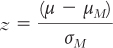 (for a distribution of means)
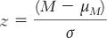 (for a distribution of means)
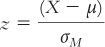 (for a distribution of scores)
Calculating the Statistics
Question 6.15
| 6.15 |
Create a histogram for these three sets of scores. Each set of scores represents a sample taken from the same population.
|
150
Question 6.16
| 6.16 |
A population has a mean of 250 and a standard deviation of 47. Calculate z scores for each of the following raw scores:
|
Question 6.17
| 6.17 |
A population has a mean of 1179 and a standard deviation of 164. Calculate z scores for each of the following raw scores:
|
Question 6.18
| 6.18 |
For a population with a mean of 250 and a standard deviation of 47, calculate the z score for 250. Explain the meaning of the value you obtain. |
Question 6.19
| 6.19 |
For a population with a mean of 250 and a standard deviation of 47, calculate the z scores for 203 and 297. Explain the meaning of these values. |
Question 6.20
| 6.20 |
For a population with a mean of 250 and a standard deviation of 47, convert each of the following z scores to raw scores.
|
Question 6.21
| 6.21 |
For a population with a mean of 1179 and a standard deviation of 164, convert each of the following z scores to raw scores.
|
Question 6.22
| 6.22 |
By design, the verbal subtest of the Graduate Record Examination (GRE) has a population mean of 500 and a population standard deviation of 100. Convert the following z scores to raw scores without using a formula.
|
Question 6.23
| 6.23 |
By design, the verbal subtest of the Graduate Record Examination (GRE) has a population mean of 500 and a population standard deviation of 100. Convert the following z scores to raw scores using symbolic notation and the formula.
|
Question 6.24
| 6.24 |
A study of the Consideration of Future Consequences (CFC) scale found a mean score of 3.20, with a standard deviation of 0.70, for the 800 students in the sample (Adams, 2012). (Treat this sample as the entire population of interest.)
|
Question 6.25
| 6.25 |
Using the instructions in Example 6.8, compare the following “apples and oranges”: a score of 45 when the population mean is 51 and the standard deviation is 4, and a score of 732 when the population mean is 765 and the standard deviation is 23.
|
Question 6.26
| 6.26 |
Compare the following scores:
|
Question 6.27
| 6.27 |
Assume a normal distribution when answering the following questions.
|
Question 6.28
| 6.28 |
Compute the standard error (σM) for each of the following sample sizes, assuming a population mean of 100 and a standard deviation of 20:
|
Question 6.29
| 6.29 |
A population has a mean of 55 and a standard deviation of 8. Compute μM and σM for each of the following sample sizes:
|
151
Question 6.30
| 6.30 |
Compute a z statistic for each of the following, assuming the population has a mean of 100 and a standard deviation of 20:
|
Question 6.31
| 6.31 |
A sample of 100 people had a mean depression score of 85; the population mean for this depression measure is 80, with a standard deviation of 20. A different sample of 100 people had a mean score of 17 on a different depression measure; the population mean for this measure is 15, with a standard deviation of 5.
|
Applying the Concepts
Question 6.32
| 6.32 |
Normal distributions in real life: Many variables are normally distributed, but not all are. (Fortunately, the central limit theorem saves us when we conduct research on samples from nonnormal populations if the samples are larger than 30!) Which of the following are likely to be normally distributed, and which are likely to be nonnormal? Explain your answers.
|
Question 6.33
| 6.33 |
Distributions and getting ready for a date: We asked 150 students in our statistics classes how long, in minutes, they typically spend getting ready for a date. The scores ranged from 1 minute to 120 minutes, and the mean was 51.52 minutes. Here are the data for 40 of these students:
|
Question 6.34
| 6.34 |
z scores and the GRE: By design, the verbal subtest of the GRE has a population mean of 500 and a population standard deviation of 100 (the quantitative subtest has the same mean and standard deviation).
|
Question 6.35
| 6.35 |
The z distribution and hours slept: A sample of 150 statistics students reported the typical number of hours that they sleep on a weeknight. The mean number of hours was 6.65, and the standard deviation was 1.24. (For this exercise, treat this sample as the entire population of interest.)
|
Question 6.36
| 6.36 |
The z distribution applied to admiration ratings: A sample of 148 of our statistics students rated their level of admiration for Hillary Clinton on a scale of 1 to 7. The mean rating was 4.06, and the standard deviation was 1.70. (For this exercise, treat this sample as the entire population of interest.) 152
|
Question 6.37
| 6.37 |
z statistics and CFC scores: We have already discussed summary parameters for CFC scores for the population of participants in a study by Adams (2012). The mean CFC score was 3.20, with a standard deviation of 0.70. (Remember that we treated the sample of 800 participants as the entire population.) Imagine that you randomly selected 40 people from this population and had them watch a series of videos on financial planning after graduation. The mean CFC score after watching the video was 3.62.
|
Question 6.38
| 6.38 |
Converting z scores to raw CFC scores: A study using the Consideration of Future Consequences scale found a mean CFC score of 3.20, with a standard deviation of 0.70, for the 800 students in the sample (Adams, 2012).
|
Question 6.39
| 6.39 |
The normal curve and real-
|
Question 6.40
| 6.40 |
The normal curve and real-
|
Question 6.41
| 6.41 |
The normal curve in the media: Statistics geeks rejoiced when the New York Times published an article on the normal curve (Dunn, 2013)! Biologist Casey Dunn wrote that “Many real- |
Question 6.42
| 6.42 |
Percentiles and eating habits: As noted in How It Works 6.1, Georgiou and colleagues (1997) reported that college students had healthier eating habits, on average, than did those who were neither college students nor college graduates. The 412 students in the study ate breakfast a mean of 4.1 times per week, with a standard deviation of 2.4. (For this exercise, again imagine that this is the entire population of interest.)
|
Question 6.43
| 6.43 |
z scores and comparisons of sports teams: A common quandary faces sports fans who live in the same city but avidly follow different sports. How does one determine whose team did better with respect to its league division? In 2012, the Atlanta Braves baseball team and the Atlanta Falcons football team both did well. The Braves won 94 games and the Falcons won 13. Which team was better in 2012? The question, then, is: Were the Braves better, as compared to the other teams in Major League Baseball (MLB), than the Falcons, as compared to the other teams in the National Football League (NFL)? Some of us could debate this for hours, but it’s better to examine some statistics. Let’s operationalize performance over the season as the number of wins during regular season play. 153
|
Question 6.44
| 6.44 |
z scores and comparisons of admiration ratings: Our statistics students were asked to rate their admiration of Hillary Clinton on a scale of 1 to 7. They also were asked to rate their admiration of actor, singer, and former American Idol judge Jennifer Lopez and their admiration of tennis player Venus Williams on a scale of 1 to 7. As noted earlier, the mean rating of Clinton was 4.06, with a standard deviation of 1.70. The mean rating of Lopez was 3.72, with a standard deviation of 1.90. The mean rating of Williams was 4.58, with a standard deviation of 1.46. One of our students rated her admiration of Clinton and Williams at 5 and her admiration of Lopez at 4.
|
Question 6.45
| 6.45 |
Raw scores, z scores, percentiles, and sports teams: Let’s look at baseball and football again. We’ll look at data for all of the teams in Major League Baseball (MLB) and the National Football League (NFL), respectively.
|
Question 6.46
| 6.46 |
Distributions and life expectancy: Researchers have reported that the projected life expectancy for South African men diagnosed with human immunodeficiency virus (HIV) at age 20 who receive antiretroviral therapy (ART) is 27.6 years ( Johnson et al., 2013). Imagine that the researchers determined this by following 250 people with HIV who were receiving ART and calculating the mean.
|
Question 6.47
| 6.47 |
Distributions, personality testing, and depression: The revised version of the Minnesota Multiphasic Personality Inventory (MMPI-
|
Question 6.48
| 6.48 |
Distributions, personality testing, and social introversion: See the description of the MMPI-
|
Question 6.49
| 6.49 |
Distributions and the General Social Survey: The General Social Survey (GSS) is a survey of approximately 2000 adults conducted each year since 1972, for a total of more than 38,000 participants. During several years of the GSS, participants were asked how many close friends they have. The mean for this variable is 7.44 friends, with a standard deviation of 10.98. The median is 5.00 and the mode is 4.00.
|
Question 6.50
| 6.50 |
A distribution of scores and the General Social Survey: Refer to Exercise 6.49. Again, pretend that the GSS sample is the entire population of interest.
|
Question 6.51
| 6.51 |
A distribution of means and the General Social Survey: Refer to Exercise 6.49. Again, pretend that the GSS sample is the entire population of interest.
|
Question 6.52
| 6.52 |
Percentiles, raw scores, and credit card theft: Credit card companies will often call cardholders if the pattern of use indicates that the card might have been stolen. Let’s say that you charge an average of $280 a month on your credit card, with a standard deviation of $75. The credit card company will call you anytime your purchases for the month exceed the 98th percentile. What is the dollar amount beyond which you’ll get a call from your credit card company? |
Putting It All Together
Question 6.53
| 6.53 |
Probability and medical treatments: The three most common treatments for blocked coronary arteries are medication; bypass surgery; and angioplasty, which is a medical procedure that involves clearing out arteries and that leads to higher profits for doctors than do the other two procedures. The highest rate of angioplasty in the United States is in Elyria, a small city in Ohio. A 2006 article in the New York Times stated that “the statistics are so far off the charts— 155
|
Question 6.54
| 6.54 |
Rural friendships and the General Social Survey: Earlier, we considered data from the GSS on numbers of close friends people reported having. The mean for this variable is 7.44, with a standard deviation of 10.98. Let’s say that you decide to use the GSS data to test whether people who live in rural areas have a different mean number of friends than does the overall GSS sample. Again, treat the overall GSS sample as the entire population of interest. Let’s say that you select 40 people living in rural areas and find that they have an average of 3.9 friends.
|
Question 6.55
| 6.55 |
Cheating on standardized tests: In their book Freakonomics, Levitt and Dubner (2009) describe alleged cheating among teachers in the Chicago public school system. Certain classrooms had suspiciously strong performances on standardized tests that often mysteriously declined the following year when a new teacher taught the same students. In about 5% of classrooms studied, Levitt and other researchers found blocks of correct answers, among most students, for the last few questions, an indication that the teacher had changed responses to difficult questions for most students. Let’s assume cheating in a given classroom if the overall standardized test score for the class showed a surprising change from one year to the next.
|