nolanessentials3e

7.1 The z Table

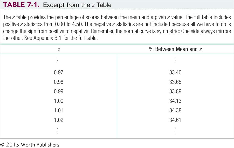
In Chapter 6, we learned that (1) about 68% of scores fall within one z score of the mean, (2) about 96% of scores fall within two z scores of the mean, and (3) nearly all scores fall within three z scores of the mean. These guidelines are useful, but the table of z statistics and percentages is more specific. The z table is printed in its entirety in Appendix B.1 but, for your convenience, we have provided an excerpt in Table 7-1. In this section, we learn how to use the z table to calculate percentages when the z score is not a whole number.

Raw Scores, z Scores, and Percentages

Just as the same person might be called variations of a single name—“Christina,” “Christy,” or “Tina,” for instance—z scores are just one of three different ways to identify the same point beneath the normal curve: raw score, z score, and percentile ranking. The z table is how we transition from one way of naming a score to another. More importantly, the z table gives us a way to state and test hypotheses by standardizing different kinds of observations onto the same scale.

159

MASTERING THE CONCEPT

7-1: We can use the z table to look up the percentage of scores between the mean of the distribution and a given z statistic.

For example, we can determine the percentage associated with a given z statistic by following two steps.

Step 1: Convert a raw score into a z score.

Step 2: Look up a given z score on the z table to find the percentage of scores between the mean and that z score.

Note that the z scores displayed in the z table are all positive, but that is just to save space. The normal curve is symmetric, so negative z scores (any scores below the mean) are the mirror image of positive z scores (any scores above the mean) (Figure 7-1).

Figure 7.2: FIGURE 7-1
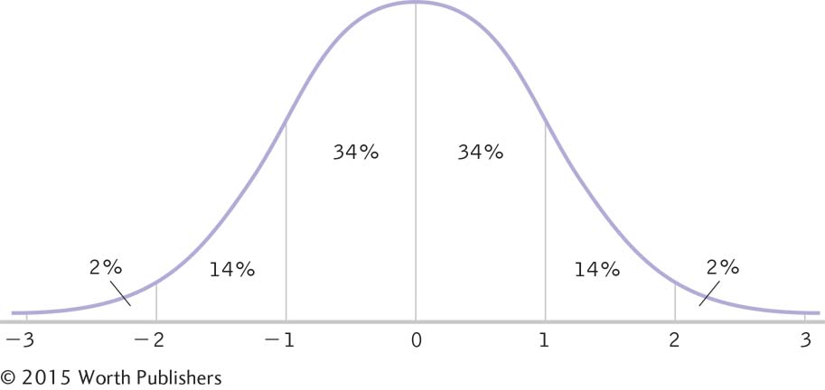
The Standardized z Distribution
We can use a z table to determine the percentages below and above a particular z score. For example, 34% of scores fall between the mean and a z score of 1.

EXAMPLE 7.1

160

Here is an interesting way to learn how to use the z table: A research team (Sandberg, Bukowski, Fung, & Noll, 2004) wanted to know whether very short children tended to have poorer psychological adjustment than taller children and, therefore, should be treated with growth hormone. They categorized 15-year-old boys and girls into one of three groups—short (bottom 5%), average (middle 90%), or tall (top 5%)—based on published norms for a given age and gender (Centers for Disease Control National Center for Health Statistics, 2000; Sandberg et al., 2004). The mean height for 15-year-old boys was approximately 67.00 inches, with a standard deviation of 3.19. For 15-year-old girls, the mean height was approximately 63.80 inches, with a standard deviation of 2.66. We’ll consider two 15-year-olds, one taller than average and the other shorter than average.

Jessica is 66.41 inches tall (just over 5 feet, 6 inches).

STEP 1: Convert her raw score to a z score, as we learned how to do in Chapter 6.

We use the mean (μ = 63.80) and standard deviation (σ = 2.66) for the heights of girls:

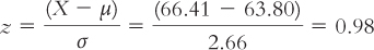
STEP 2: Look up 0.98 on the z table to find the associated percentage between the mean and Jessica’s z score.

Once we know that the associated percentage is 33.65%, we can determine a number of percentages related to her z score. Here are three.

Jessica’s percentile rank—the percentage of scores below her score: We add the percentage between the mean and the positive z score to 50%, which is the percentage of scores below the mean (50% of scores are on each side of the mean).

Jessica’s percentile is 50% + 33.65% = 83.65%

Figure 7-2 shows this visually. As we can do when we are evaluating the calculations of z scores, we can run a quick mental check of the likely accuracy of the answer. We’re interested in calculating the percentile of a positive z score. Because it is above the mean, we know that the answer must be higher than 50%. And it is.

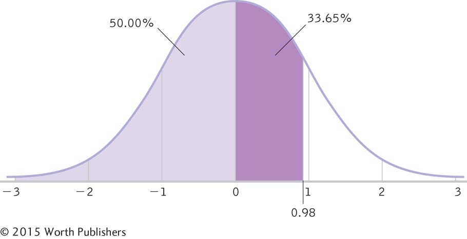Figure 7.3: FIGURE 7-2
Calculating the Percentile for a Positive z Score
Drawing curves helps us find someone’s percentile rank. For Jessica’s positive z score of 0.98, add the 50% below the mean to the 33.65% between the mean and her z score of 0.98; Jessica’s percentile rank is 83.65%.

161
The percentage of scores above Jessica’s score: We subtract the percentage between the mean and the positive z score from 50%, which is the full percentage of scores above the mean:

50% – 33.65% = 16.35%

So 16.35% of 15-year-old girls’ heights are above Jessica’s height. Figure 7-3 shows this visually. Here, it makes sense that the percentage would be smaller than 50%; because the z score is positive, we could not have more than 50% above it. As an alternative, a simpler method is to subtract Jessica’s percentile rank of 83.65% from 100%. This gives us the same 16.35%. We could also look under the “In the tail” column in the z table in Appendix B.1.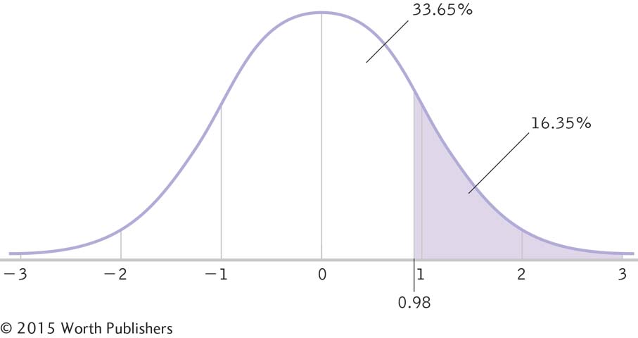

Figure 7.4: FIGURE 7-3
Calculating the Percentage Above a Positive z Score
For a positive z score, we subtract the percentage between the mean and that z score from 50% (the total percentage above the mean) to get the percentage above that z score. Here, we subtract the 33.65% between the mean and the z score of 0.98 from 50%, which yields 16.35%.
The scores at least as extreme as Jessica’s z score, in both directions: When we begin hypothesis testing, it will be useful to know the percentage of scores that are at least as extreme as a given z score. In this case, 16.35% of heights are extreme enough to have z scores above Jessica’s z score of 0.98. But remember that the curve is symmetric. This means that another 16.35% of the heights are extreme enough to be below a z score of –0.98. So we can double 16.35% to find the total percentage of heights that are as far as or farther from the mean than is Jessica’s height:

16.35% + 16.35% = 32.70%

Thus 32.7% of heights are at least as extreme as Jessica’s height in either direction. Figure 7-4 shows this visually.

Figure 7.5: FIGURE 7-4
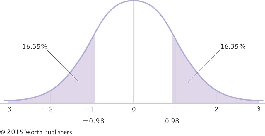
Calculating the Percentage at Least as Extreme as the z Score
For a positive z score, we double the percentage above that z score to get the percentage of scores that are at least as extreme—that is, at least as far from the mean—as the z score is. Here, we double 16.35% to calculate the percentage at least this extreme: 32.70%.

What group would Jessica fall in? Because 16.35% of 15-year-old girls are taller than Jessica, she is not in the top 5%. So she would be classified as being of average height, according to the researchers’ definition of average.

162

EXAMPLE 7.2

Now let’s repeat this process for a score below the mean. Manuel is 61.20 inches tall (about 5 feet, 1 inch) so we want to know if Manuel can be classified as short. Remember, for boys the mean height is 67.00 inches, and the standard deviation for height is 3.19 inches.

STEP 1: Convert his raw score to a z score:

We use the mean ( μ = 67.00) and standard deviation (σ = 3.19) for the heights of boys:

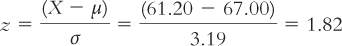
STEP 2: Calculate the percentile, the percentage above, and the percentage at least as extreme for the negative z score for Manuel’s height.

We can again determine a number of percentages related to the z score; however, this time, we need to use the full table in Appendix B. The z table includes only positive z scores, so we look up 1.82 and find that the percentage between the mean and the z score is 46.56%. Of course, percentages are always positive, so don’t add a negative sign here!

Manuel’s percentile score—the percentage of scores below his score: For a negative z score, we subtract the percentage between the mean and the z score from 50% (which is the total percentage below the mean):

Manuel’s percentile is 50% – 46.5% = 3.44% (Figure 7-5).

Figure 7.6: FIGURE 7-5
Calculating the Percentile for a Negative z Score
As with positive z scores, drawing curves helps us to determine the appropriate percentage for negative z scores. For a negative z score, we subtract the percentage between the mean and that z score from 50% (the percentage below the mean) to get the percentage below that negative z score, the percentile. Here we subtract the 46.56% between the mean and the z score of –1.82 from 50%, which yields 3.44%.
The percentage of scores above Manuel’s score: We add the percentage between the mean and the negative z score to 50%, the percentage above the mean:

50% + 46.56% = 96.56%

So 96.56% of 15-year-old boys’ heights fall above Manuel’s height (Figure 7-6).

163

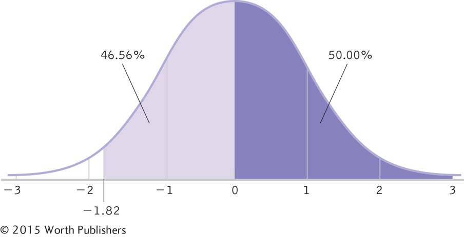Figure 7.7: FIGURE 7-6
Calculating the Percentage Above a Negative z Score
For a negative z score, we add the percentage between the mean and that z score to 50% (the percentage above the mean) to get the percentage above that z score. Here we add the 46.56% between the mean and the z score of –1.82 to the 50% above the mean, which yields 96.56%.
The scores at least as extreme as Manuel’s z score, in both directions: In this case, 3.44% of 15-year-old boys have heights that are extreme enough to have z scores below –1.82. And because the curve is symmetric, another 3.44% of heights are extreme enough to be above a z score of 1.82. So we can double 3.44% to find the total percentage of heights that are as far as or farther from the mean than is Manuel’s height:

3.44% + 3.44% = 6.88%

So 6.88% of heights are at least as extreme as Manuel’s in either direction (Figure 7-7).

Figure 7.8: FIGURE 7-7
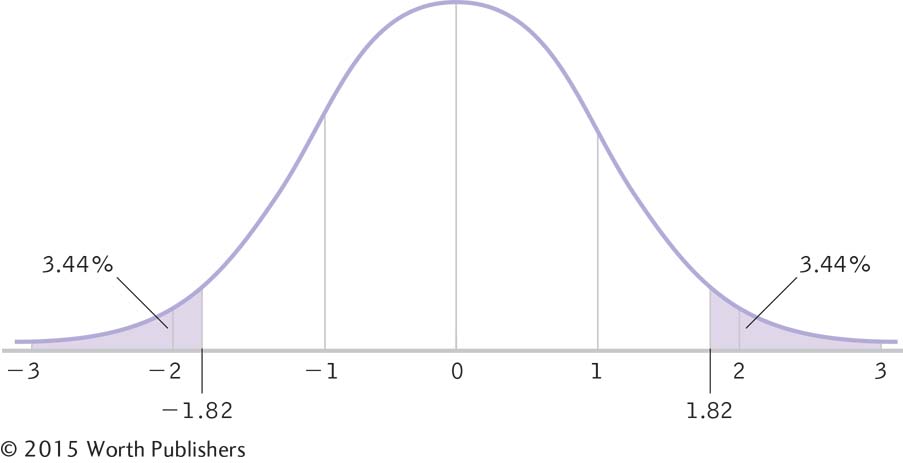
Calculating the Percentage at Least as Extreme as the z Score
With a negative z score, we double the percentage below that z score to get the percentage of scores that are at least as extreme—that is, at least as far from the mean—as the z score is. Here, we double 3.44% to calculate the percentage at least this extreme: 6.88%.

In what group would the researchers classify Manuel? Manuel has a percentile rank of 3.44%. He is in the lowest 5% of heights for boys of his age, so he would be classified as short. Now we can get to the question that drives this research. Does Manuel’s short stature doom him to a life of few friends and poor social adjustment? Researchers compared the means of the three groups—short, average, and tall—on several measures of peer relations and social adjustment, but they did not find evidence of mean differences among the groups (Sandberg et al., 2004).

EXAMPLE 7.3

This example demonstrates (a) how to seamlessly shift among raw scores, z scores, and percentile ranks; and (b) why drawing a normal curve makes the calculations much easier to understand.

Many high school students in North America take the Scholastic Aptitude Test (SAT). The parameters for each part of the SAT are set at a mean of 500 and a standard deviation of 100. So let’s imagine that Jo, a high school student hoping to attend college, took the SAT and scored at the 63rd percentile on one part. What was her raw score? Begin by drawing a curve, as in Figure 7-8. Then add a line at the point below which approximately 63% of scores fall. We know that this score is above the mean because 50% of scores fall below the mean, and 63% is larger than 50%.

164

Figure 7.9: FIGURE 7-8
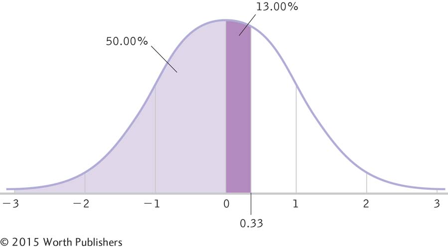
Calculating a Score from a Percentile
We convert a percentile to a raw score by calculating the percentage between the mean and the z score, and then looking up that percentage on the z table to find the associated z score. We then convert the z score to a raw score using the formula. Here, we look up 13.00% on the z table (12.93% is the closest percentage) and find a z score of 0.33, which we can convert to a raw score.

Using the drawing as a guideline, we see that we have to calculate the percentage between the mean and the z score of interest. So, we subtract the 50% below the mean from Jo’s score, 63%:

63% – 50% = 13%

We look up the closest percentage to 13% in the z table (which is 12.93%) and find an associated z score of 0.33. This is above the mean, so we do not label it with a negative sign. We then convert the z score to a raw score using the formula we learned in Chapter 6:

X = z(σ) + μ = 0.33(100) + 500 = 533

Jo, whose SAT score was at the 63rd percentile, had a raw score of 533. Double check! This score is above the mean of 500, and the percentage is above 50%.

The z Table and Distributions of Means

Let’s shift our focus from the z score of an individual within a group to the z statistic for a group. There are a couple changes to the calculations. First, we will use means rather than individual scores because we are now studying a sample of many scores rather than studying one individual score. Fortunately, the z table can also be used to determine percentages and z statistics for distributions of means calculated from many people. The other change is that we need to calculate the mean and the standard error for the distribution of means before calculating the z statistic.

EXAMPLE 7.4

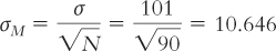
Many psychology graduate programs require that applicants take the Graduate Record Exam (GRE) subject test in psychology. The test has been used for many years, so we know the actual population mean and standard deviation. For example, the mean was 603 and the standard deviation was 101 for one recent year, numbers that we will treat as population parameters for this example (http://nces.ed.gov/programs/digest/d12/tables/dt12_380.asp). z statistics make it possible to compare psychology students at our institution to that known standard. We record the psychology test scores of a representative sample, 90 graduating seniors in a psychology department, and find that the mean score is 622. Before we calculate the z statistic, let’s use proper symbolic notation to indicate the mean and the standard error of this distribution of means:

165

μ_M = μ = 603

At this point, we have all the information we need to calculate the percentage using the two steps we learned earlier.

STEP 1: We convert to a z statistic using the mean and standard error that we just calculated.

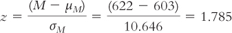
STEP 2: We determine the percentage below this z statistic.

Draw it! Draw a curve that includes the mean of the z distribution, 0, and this z statistic, 1.785, rounded to 1.79 (Figure 7-9). Then shade the area in which we are interested: everything below 1.79. Now we look up the percentage between the mean and the z statistic of 1.79. The z table indicates that this percentage is 46.33, which we write in the section of the curve between the mean and 1.79. We write 50% in the half of the curve below the mean. We add 46.33% to the 50% below the mean to get the percentile rank, 96.33%. (Subtracting from 100%, only 3.67% of mean scores would be higher than the mean if they come from this population.) Based on this percentage, the mean GRE psychology test score of the sample is quite high. But we still can’t arrive at a conclusion about whether these students are performing above the national average of 603 until we conduct a hypothesis test.

Figure 7.10: FIGURE 7-9
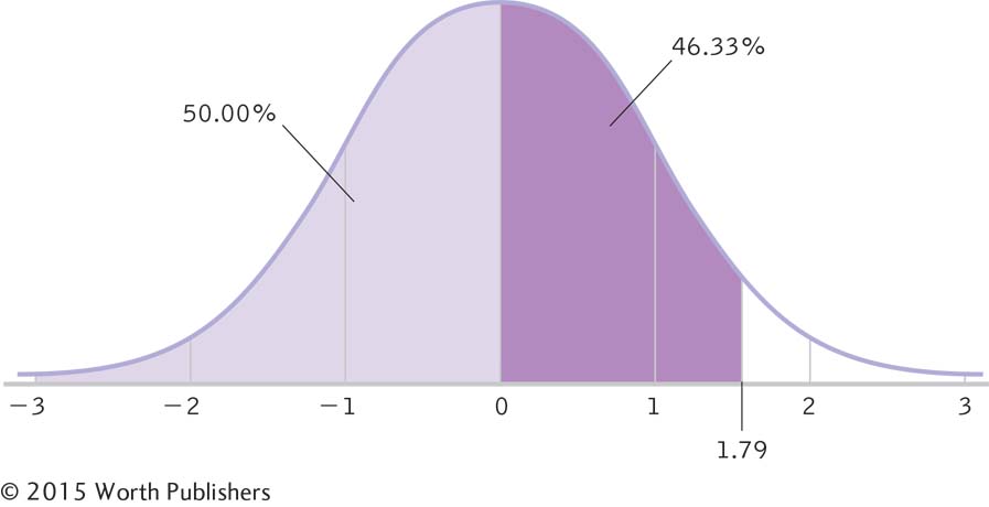
Percentile for the Mean of a Sample
We can use the z table with sample means in addition to sample scores. The only difference is that we use the mean and standard error of the distribution of means rather than the distribution of scores. Here, the z score of 1.79 is associated with a percentage of 46.33% between the mean and z score. Added to the 50% below the mean, the percentile is 50% + 46.33% = 96.33%.

166

In the next section, we learn (a) the assumptions for conducting hypothesis testing; (b) the six steps of hypothesis testing using the z distribution; and (c) whether to reject or fail to reject the null hypothesis. In the last section, we demonstrate a z test.

CHECK YOUR LEARNING

Reviewing the Concepts		Raw scores, z scores, and percentile rankings are three ways to describe the same score within a normal distribution. If we know the mean and the standard deviation of a population, we can convert a raw score to a z score and then use the z table to determine percentages below, above, or at least as extreme as this z score. We can use the z table in reverse as well, taking a percentage and converting it into a z score and then a raw score. These same conversions can be conducted on a sample mean instead of on a score. The procedures are identical, but we use the mean and the standard error of the distribution of means, instead of the distribution of scores.
Clarifying the Concepts	7-1	What information do we need to know about a population of interest in order to use the z table?
	7-2	How do z scores relate to raw scores and percentile ranks?
Calculating the Statistics	7-3	If the percentage of scores between a z score of 1.37 and the mean is 41.47%, what percentage of scores lies between –1.37 and the mean?
	7-4	If 12.93% of scores fall between the mean and a z score of 0.33, what percentage of scores falls below this z score?
Applying the Concepts	7-5	Every year, the Educational Testing Service (ETS) administers the Major Field Test in Psychology (MFTP) to graduating psychology majors. Baylor University wondered how its students compared to the national average. On its Web site, Baylor reported that the mean and the standard deviation of the 18,073 U.S. students who took this exam were 156.8 and 14.6, respectively. Thirty-six students in Baylor’s psychology and neuroscience department took the exam; these students had a mean score of 164.6.
		What is the percentile rank for the sample of students at Baylor? Use symbolic notation and write out your calculations. What percentage of samples of this size scored higher, on average, than the students at Baylor? What can you say about how Baylor students compared to students across the nation?

Solutions to these Check Your Learning questions can be found in Appendix D.