Chapter 10
- 10.1 We can understand the meaning of a distribution of mean differences by reviewing how the distribution is created in the first place. A distribution of mean differences is constructed by measuring the difference scores for a sample of individuals and then averaging those differences. This process is performed repeatedly, using the same population and samples of the same size. Once a collection of mean differences is gathered, they can be displayed on a graph (in most cases, they form a bell-
shaped curve). - 10.3 The term paired samples is used to describe a test that compares an individual’s scores in both conditions; it is also called a paired-samples t test. Independent samples refer to groups that do not overlap in any way, including membership; the observations made in one group in no way relate to or depend on the observations made in another group.
- 10.5 Unlike a single-
sample t test, in the paired- samples t test we have two scores for every participant; we take the difference between these scores before calculating the sample mean difference that will be used in the t test. - 10.7 If the confidence interval around the mean difference score includes the value of 0, then 0 is a plausible mean difference. If we conduct a hypothesis test for these data, we would fail to reject the null hypothesis.
- 10.9 As with other hypothesis tests, the conclusions from both the single-
sample t test or paired- samples t test and the confidence interval are the same, but the confidence interval gives us more information— an interval estimate, not just a point estimate. - 10.11 Order effects occur when performance on a task changes because the dependent variable is being presented for a second time.
- 10.13 Because order effects result in a change in the dependent variable that is not directly the result of the independent variable of interest, the researcher may decide to use a between-
groups design, particularly when counterbalancing is not possible. For example, a researcher may be interested in how the amount of practice affects the acquisition of a new language. It would not be possible for the same participants to be in both a group that has small amounts of practice and a group that has large amounts of practice. - 10.15
- a. df = 17, so the critical t value is +2.567, assuming you’re anticipating an increase in marital satisfaction.
- b. df = 63, so the critical t values are ±2.001.
- 10.17
- a.
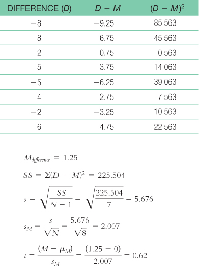
- b. With df = 7, the critical t values are ±2.365. The calculated t statistic of 0.62 does not exceed the critical value. Therefore, we fail to reject the null hypothesis.
- c. When increasing N to 1000, we need to recalculate sM and the t test.
- d. Increasing the sample size increased the value of the t statistic and decreased the critical t values, making it easier for us to reject the null hypothesis.
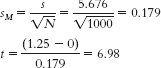
The critical values with df = 7 are t = ±1.98. Because the calculated t exceeds one of the t critical values, we reject the null hypothesis. - a.
- 10.19
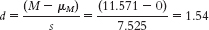
- a.
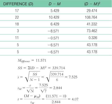
- b. With N = 7, df = 6, t = ±2.447:
Mlower = −t(sM) + Msample = −2.447(2.844) + 11.571 = 4.61
Mupper = t(sM) + Msample = 2.447(2.844) + 11.571 = 18.53 - c.
- a.
- 10.21
- a.
C-
29 - b.
- c.
- a.
- 10.23 A study using a paired-
samples t test design would compare people before and after training using the program of mental exercises designed by PowerBrainRx. Population 1 would be participants before the mental exercises training. Population 2 would be participants after the mental exercises training.
The comparison distribution is a distribution of mean differences. The participants receiving mental exercises training are the same in both samples. So, we would calculate a difference score for each participant and a mean difference score for the study. The mean difference score would be compared to a distribution of all possible mean difference scores for a sample of this size and based on the null hypothesis. In this case, the mean difference score would be compared to zero. Because we have two samples and all participants are in both samples, we would use a paired-samples t test. - 10.25
- a. Step 1: Population 1 is the Devils players in the 2007–
2008 season. Population 2 is the Devils players in the 2008– 2009 season. The comparison distribution is a distribution of mean differences. We meet one assumption: The dependent variable, goals, is scale. We do not, however, meet the assumption that the participants are randomly selected from the population. We may also not meet the assumption that the population distribution of scores is normally distributed (the scores do not appear normally distributed and we do not have an N of at least 30).
Step 2: Null hypothesis: The team performed no differently, on average, between the 2007–2008 and 2008– 2009 seasons— H0: μ1 = μ2.
Research hypothesis: The team scored a different number of goals, on average, between the 2007–2008 and 2008– 2009 seasons— H1: μ1 ≠ μ2.
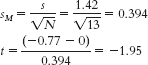
Step 3: μ = 0 and sM = 3.682Step 4: The critical t values with a two-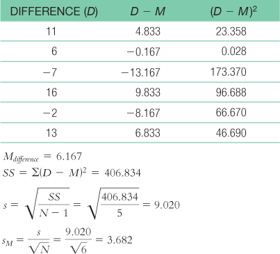
tailed test, a p level of 0.05, and 5 degrees of freedom, are +2.571.
Step 5: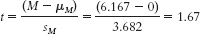
Step 6: Fail to reject the null hypothesis because the calculated t statistic of 1.67 does not exceed the critical t value. - b. t(5) = 1.67, p > 0.05 (Note: If we had used software, we would provide the actual p value.)
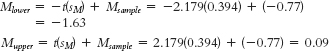
- c.
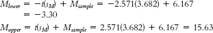
Because the confidence interval includes 0, we fail to reject the null hypothesis. This is consistent with the results of the hypothesis test conducted in part (a). - d.
- a. Step 1: Population 1 is the Devils players in the 2007–
- 10.27
- a. The professor would use a paired-
samples t-test. - b. No. A change or a difference in mean score might not be statistically significant, particularly with a small sample.
- c. It would be easier to reject the null hypothesis for a given mean difference with the class with 700 students than with the class with 7 students because the t value would be higher with the larger sample.
- a. The professor would use a paired-
- 10.29
- a. The independent variable is presence of posthypnotic suggestion, with two levels: suggestion or no suggestion. The dependent variable is Stroop reaction time in seconds.
- b. Step 1: Population 1 is highly hypnotizable individuals who receive a posthypnotic suggestion. Population 2 is highly hypnotizable individuals who do not receive a posthypnotic suggestion. The comparison distribution will be a distribution of mean differences. The hypothesis test will be a paired-
samples t test because we have two samples and all participants are in both samples. This study meets one of the three assumptions and may meet another. The dependent variable, reaction time in seconds, is scale. The data were not likely randomly selected, so we should be cautious when generalizing beyond the sample. We do not know whether the population is normally distributed and there are not at least 30 participants, but the sample data do not suggest skew.
Step 2: Null hypothesis: Highly hypnotizable individuals who receive a posthypnotic suggestion will have the same average Stroop reaction times as highly hypnotizable individuals who receive no posthypnotic suggestion—H0: μ1 = μ2.
Research hypothesis: Highly hypnotizable individuals who receive a posthypnotic suggestion will have different average Stroop reaction times than will highly hypnotizable individuals who receive no posthypnotic suggestion—H1: μ1 ≠ μ2.
Step 3: μM = l = 0; sM = 0.420
(Note: Remember to cross out the original scores once you have created the difference scores so you won’t be tempted to use them in your calculations.)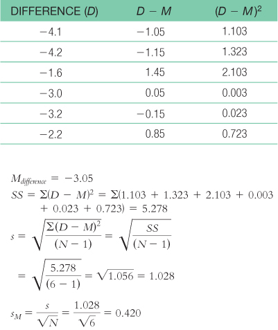 Step 4: df = N − 1 = 6 − 1 = 5; the critical values, based on 5 degrees of freedom, a p level of 0.05, and a two-
C-
30 tailed test, are −2.571 and 2.571.
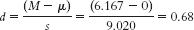
Step 5: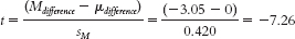
Step 6: Reject the null hypothesis; it appears that highly hypnotizable people have faster Stroop reaction times when they receive a posthypnotic suggestion than when they do not. - c. t(5) = −7.26, p < 0.05
- d. Step 2: Null hypothesis: The average Stroop reaction time of highly hypnotizable individuals who receive a posthypnotic suggestion is greater than or equal to that of highly hypnotizable individuals who receive no posthypnotic suggestion—
H0: μ1 ≥ μ2.Research hypothesis: Highly hypnotizable individuals who receive a posthypnotic suggestion will have faster (i.e., lower number) average Stroop reaction times than highly hypnotizable individuals who receive no posthypnotic suggestion— H1: μ1 < μ2.
Step 4: df = N − 1 = 6 − 1 = 5; the critical value, based on 5 degrees of freedom, a p level of 0.05, and a one-tailed test, is +2.015. (Note: It is helpful to draw a curve that includes this cutoff.)
Step 6: Reject the null hypothesis; it appears that highly hypnotizable people have faster Stroop reaction times when they receive a posthypnotic suggestion than when they do not.
It is easier to reject the null hypothesis with a one-tailed test. Although we rejected the null hypothesis under both conditions, the critical t value is less extreme with a one- tailed test because the entire 0.05 (5%) critical region is in one tail instead of divided between two.
The difference between the means of the samples is identical, as is the test statistic. The only aspect that is affected is the critical value. - e. Step 4: df = N − 1 = 6 − 1 = 5; the critical values, based on 5 degrees of freedom, a p level of 0.01, and a two-
tailed test, are −4.032 and 4.032. (Note: It is helpful to draw a curve that includes these cutoffs.)Step 6: Reject the null hypothesis; it appears that highly hypnotizable people have faster mean Stroop reaction times when they receive a posthypnotic suggestion than when they do not.
A p level of 0.01 leads to more extreme critical values than a p level of 0.05. When the tails are limited to 1% versus 5%, the tails beyond the cutoffs are smaller and the cutoffs are more extreme. So it is easier to reject the null hypothesis with a p level of .05 than the null hypothesis with a p level of .01.
The difference between the means of the samples is identical, as is the test statistic. The only aspect that is affected is the critical value. - f. Step 3: μM = μ = 0; sM = 0.850(Note: Remember to cross out the original scores once you have created the difference scores so you won’t be tempted to use them in your calculations.)Step 4: df = N − 1 = 3 − 1 = 2; the critical values, based on 2 degrees of freedom, a p level of 0.05, and a two-
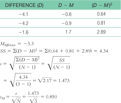
tailed test, are −4.303 and 4.303. (Note: It is helpful to draw a curve that includes these cutoffs.)
Step 5: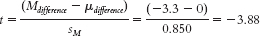
(Note: It is helpful to add this t statistic to the curve that you drew in step 4.)
This test statistic is no longer beyond the critical value. Reducing the sample size makes it more difficult to reject the null hypothesis because it results in a larger standard error and therefore a smaller test statistic. It also results in more extreme critical values. - g. Participants might get faster at completing the Stroop test as a result of practice with it. If so, their reaction times would be faster the second time they complete the task regardless of whether they had the posthypnotic suggestion.
- h. The researchers could not use counterbalancing because this was a pre–
post design. However, one way to get rid of possible order effects would be to use a between- groups design in which some participants are given the posthypnotic suggestion but others are not, and to compare the means of these two groups.