nolanheinzen3e

Chapter 11

11.1 An independent-samples t test is used when we do not know the population parameters and are comparing two groups that are composed of unrelated participants or observations.
11.3 Independent events are things that do not affect each other. For example, the lunch you buy today does not impact the hours of sleep the authors of this book will get tonight.
11.5 The comparison distribution for the paired-samples t test is made up of mean differences—the average of many difference scores. The comparison distribution for the independent-samples t test is made up of differences between means, or the differences we can expect to see between group means if the null hypothesis is true.
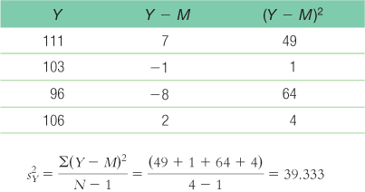
C-31
11.7 Both of these represent corrected variance within a group (s²), but one is for the X variable and the other is for the Y variable. Because these are corrected measures of variance, N − 1 is in the denominator of the equations.
11.9 We assume that larger samples do a better job of estimating the population than smaller samples do, so we would want the variability measure based on the larger sample to count more.
11.11 We can take the confidence interval’s upper bound and lower bound, compare those to the point estimate in the numerator, and get the margin of error. So, if we predict a score of 7 with a confidence interval of [4.3, 9.7], we can also express this as a margin of error of 2.7 points (7 ± 2.7). Confidence interval and margin of error are simply two ways to say the same thing.
11.13 Larger ranges mean less precision in making predictions, just as widening the goal posts in rugby or in American football mean that you can be less precise when trying to kick the ball between the posts. Smaller ranges indicate we are doing a better job of predicting the phenomenon within the population. For example, a 95% confidence interval that spans a range from 2 to 12 is larger than a 95% confidence interval from 5 to 6. Although the percentage range has stayed the same, the width of the distribution has changed.
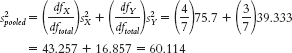
11.15 We would take several steps back from the final calculation of standard error to the step in which we calculated pooled variance. Pooled variance is the variance version, or squared version, of standard deviation. To convert pooled variance to the pooled standard deviation, we take its square root.
11.17 Guidelines for interpreting the size of an effect based on Cohen’s d were presented in Table 11-2. Those guidelines state that 0.2 is a small effect, 0.5 is a medium effect, and 0.8 is a large effect.
11.19 The square root transformation compresses both the negative and positive sides of a distribution.
11.21
- a. Group 1 is treated as the X variable; M_X = 95.8.
  
  Group 2 is treated as the Y variable; M_Y = 104
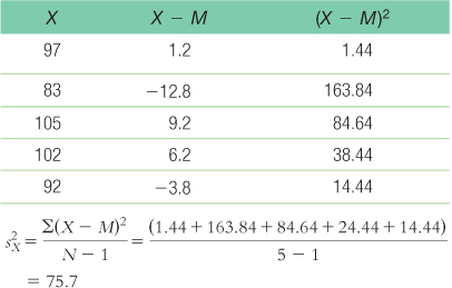
- b. Treating group 1 as X and group 2 as Y, df_X = N − 1 = 5 − 1 = 4, df_Y = 4 − 1 = 3, and df_total = df_X + df_Y = 4 + 3 = 7.
- c. −2.365, +2.365
- d.
- e. For group 1: For group 2:
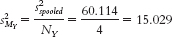
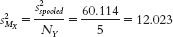
- f.
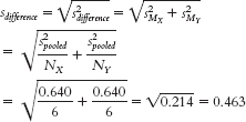
  The standard deviation of the distribution of differences between means is:
- g.
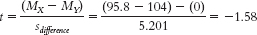
- h. The critical t values for the 95% confidence interval for a df of 7 are −2.365 and 2.365.
  
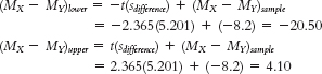
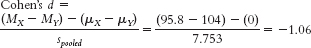
  The confidence interval is [−20.50, 4.10].
- i. To calculate Cohen’s d, we need to calculate the pooled standard deviation for the data:
11.23
- a. df_total is 35, and the cutoffs are −2.030 and 2.030.
- b. df_total is 26, and the cutoffs are −2.779 and 2.779.
- c. −1.740 and 1.740
11.25
- a. For this set of data, we would not want to apply a transformation. The mean and the median of the data set are exactly equal (both are 20), which indicates that the data are normally distributed. Thus, there is no need to apply a data transformation.
- b. For this set of data, we may consider applying a data transformation. A comparison of the mean, which is 28.3, and the median, which is 26, suggests that there is a slight positive skew to the distribution that may warrant a data transformation.
- c. For this set of data, we would probably apply a data transformation. Comparing the mean of 78 to the median of 82.5 reveals a negative skew that may warrant the use of a data transformation.
11.27
- a. Step 1: Population 1 is highly hypnotizable people who receive a posthypnotic suggestion. Population 2 is highly hypnotizable people who do not receive a posthypnotic suggestion. The comparison distribution will be a distribution of differences between means. The hypothesis test will be an independent-samples t test because we have two samples and every participant is in only one sample. This study meets one of the three assumptions and may meet another. The dependent variable, reaction time in seconds, is scale. The data were not likely randomly selected, so we should be cautious when generalizing beyond the sample. We do not know whether the population is normally distributed, and there are fewer than 30 participants, but the sample data do not suggest skew.
  C-32
  Step 2: Null hypothesis: Highly hypnotizable individuals who receive a posthypnotic suggestion have the same average Stroop reaction times as highly hypnotizable individuals who receive no posthypnotic suggestion—H₀: μ₁ + μ₂.
  Research hypothesis: Highly hypnotizable individuals who receive a posthypnotic suggestion have different average Stroop reaction times than highly hypnotizable individuals who receive no posthypnotic suggestion—H₁: μ₁ ≠ μ₂.
  Step 3: (μ₁ − μ₂) = 0; s_difference = 0.463
  Calculations:
  
  Step 4: The critical values, based on a two-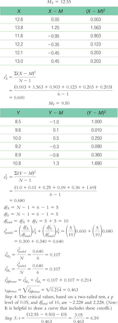tailed test, a p level of 0.05, and df_total of 10, are −2.228 and 2.228. (Note: It is helpful to draw a curve that includes these cutoffs.)
  Step 5: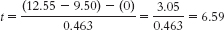
  (Note: It is helpful to add this t statistic to the curve that you drew in step 4.)
  Step 6: Reject the null hypothesis; it appears that highly hypnotizable people have faster Stroop reaction times when they receive a posthypnotic suggestion than when they do not.
- b. t(10) = 6.59, p < 0.05 (Note: If we used software to conduct the t test, we would report the actual p value associated with this test statistic.)
- c. When there are two separate samples, the t statistic becomes smaller. Thus, it becomes more difficult to reject the null hypothesis with a between-groups design than with a within-groups design.
- d. In the within-groups design and the calculation of the paired- samples t test, we create a set of difference scores and conduct a t test on that set of difference scores. This means that any overall differences that participants have on the dependent variable are subtracted out and do not go into the measure of overall variability that is in the denominator of the t statistic.
- e. To calculate the 95% confidence interval, first calculate:
  
  The critical t statistics for a distribution with df = 10 that correspond to a p level of 0.05—that is, the values that mark off the most extreme 0.025 in each tail—are −2.228 and 2.228. Then calculate:
  (M_X − M_Y)_lower = −t(s_difference) + (M_X − M_Y)_sample = −2.228(0.463) + (12.55 − 9.5) = −1.032 + 3.05 = 2.02
  (M_X − M_Y)_upper = t(s_difference) + (M_X − M_Y)_sample = 2.228(0.463) + (12.55 − 9.5) = 1.032 + 3.05 = 4.08
  The 95% confidence interval around the difference between means of 3.05 is [2.02, 4.08].
- f. Were we to draw repeated samples (of the same sizes) from these two populations, 95% of the time the confidence interval would contain the true population parameter.
- g. Because the confidence interval does not include 0, it is not plausible that there is no difference between means. Were we to conduct a hypothesis test, we would be able to reject the null hypothesis and could conclude that the means of the two samples are different.
- h. In addition to determining statistical significance, the confidence interval allows us to determine a range of plausible differences between means. An interval estimate gives us a better sense than does a point estimate of how precisely we can estimate from this study.
  C-33
- i. The appropriate measure of effect size for a t statistic is Cohen’s d, which is calculated as:
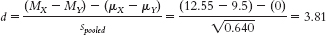
- j. Based on Cohen’s conventions, this is a large effect size.
- k. It is useful to have effect-size information because the hypothesis test tells us only whether we were likely to have obtained our sample mean by chance. The effect size tells us the magnitude of the effect, giving us a sense of how important or practical this finding is, and allows us to standardize the results of the study so that we can compare across studies. Here, we know that there’s a large effect.
11.29
- a. Step 1: Population 1 consists of men. Population 2 consists of women. The comparison distribution is a distribution of differences between means. We will use an independent- samples t test because men and women cannot be in both conditions, and we have two groups. Of the three assumptions, we meet one because the dependent variable, number of words uttered, is a scale variable. We do not know whether the data were randomly selected or whether the population is normally distributed, and there is a small N, so we should be cautious in drawing conclusions.
  Step 2: Null hypothesis: There is no mean difference in the number of words uttered by men and women—H₀: μ₁ = μ₂.
  Research hypothesis: Men and women utter a different number of words, on average—H₁: μ₁ ≠ μ₂.
  Step 3: (μ₁ − μ₂) = 0; s_difference = 612.565
  Calculations (treating women as X and men as Y):
  
  Step 4: The critical values, based on a two-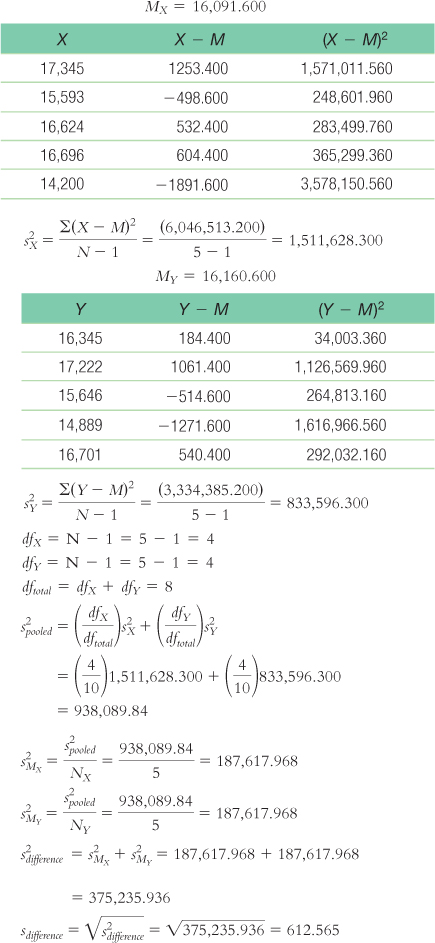tailed test, a p level of 0.05, and a df_total of 8, are −2.306 and 2.306.
  Step 5: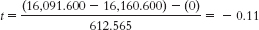
  Step 6: We fail to reject the null hypothesis. The calculated t statistic of −0.11 is not more extreme than the critical t values.
- b. t(8) = −0.11, p > 0.05 (Note: If we used software to conduct the t test, we would report the actual p value associated with this test statistic.)
- c.
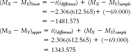
- d. The 95% confidence interval around the observed mean difference of −69.00 is [−1481.58, 1343.58].
- e. This confidence interval indicates that if we were to repeatedly sample differences between the means, 95% of the time our mean would fall between −1481.58 and 1343.58.
- f. First, we need the appropriate measure of variability. In this case, we calculate pooled standard deviation by taking the square root of the pooled variance:
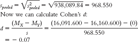
- g. This is a small effect.
- h. Effect size tells us how big the difference we observed between means was, uninfluenced by sample size. Often, this measure will help us understand whether we want to continue along our current research lines; that is, if a strong effect is indicated but we fail to reject the null hypothesis, we might want to replicate the study with more statistical power. In this case, however, the failure to reject the null hypothesis is accompanied by a small effect.
11.31
- a. Step 1: Population 1 consists of mothers, and population 2 is nonmothers. The comparison distribution will be a distribution of differences between means. We will use an independent-samples t test because someone is either identified as being a mother or not being a mother; both conditions, in this case, cannot be true. Of the three assumptions, we meet one because the dependent variable, decibel level, is a scale variable. We do not know whether the data were randomly selected and whether the population is normally distributed, and we have a small N, so we will be cautious in drawing conclusions.
  C-34
  Step 2: Null hypothesis: There is no mean difference in sound sensitivity, as reflected in the minimum level of detection, between mothers and nonmothers—H₀: μ₁ = μ₂.
  Research hypothesis: There is a mean difference in sensitivity between the two groups—H₁: μ₁ ≠ μ₂.
  Step 3: (μ₁ = μ₂) = 0; s_difference = 9.581
  Calculations:
  
  Step 4: The critical values, based on a two-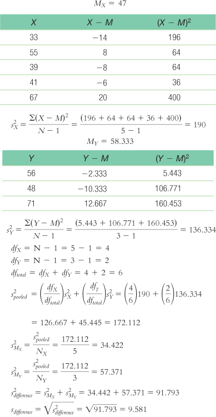tailed test, a p level of 0.05, and a df_total of 6, are −2.447 and 2.447.
  Step 5: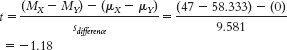
  Step 6: Fail to reject the null hypothesis. We do not have enough evidence, based on these data, to conclude that mothers have more sensitive hearing, on average, when compared to nonmothers.
- b. t(6) = −1.18, p > 0.05 (Note: If we used software to conduct the t test, we would report the actual p value associated with this test statistic.)
- c.
  
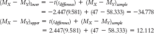
  The 95% confidence interval around the difference between means of −11.333 is [−34.78, 12.11].
- d. What we learn from this confidence interval is that there is great variability in the plausible difference between means for these data, reflected in the wide range. We also notice that 0 is within the confidence interval, so we cannot assume a difference between these groups.
- e. Whereas point estimates result in one value (−11.333 in this case) in which we have no estimate of confidence, the interval estimate gives us a range of scores about which we have known confidence.
- f.
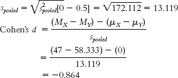
- g. This is a large effect.
- h. Effect size tells us how big the difference we observed between means was, without the influence of sample size. Often, this measure helps us decide whether we want to continue along our current research lines. In this case, the large effect would encourage us to replicate the study with more statistical power.
11.33
- a. We would use a single-sample t test because we have one sample of figure skaters and are comparing that sample to a population (women with eating disorders) for which we know the mean.
- b. We would use an independent-samples t test because we have two samples, and no participant can be in both samples. One cannot have both a high level and a low level of knowledge about a topic.
- c. We would use a paired-samples t test because we have two samples, but every student is assigned to both samples—one night of sleep loss and one night of no sleep loss.
11.35
- a. We would use an independent-samples t test because there are two samples, and no participant can be in both samples. One cannot be a pedestrian en route to work and a tourist pedestrian at the same time.
- b. Null hypothesis: People en route to work tend to walk at the same pace, on average, as people who are tourists—H₀: μ₁ = μ₂.Research hypothesis: People en route to work tend to walk at a different pace, on average, than do those who are tourists—H₁: μ₁ ≠ μ₂.
11.37
- a. The independent variable is the tray availability with levels of not available and available.
- b. The dependent variables are food waste and dish use. Food waste was likely operationalized by weight or volume of food disposed, whereas dish use was likely operationalized by number of dishes used or dirtied.
  C-35
- c. This study is an experiment because the environment was manipulated or controlled by the researchers. It assumes that the individuals were randomly sampled from the population and randomly assigned to one of the two levels of the independent variable.
- d. We would use an independent-samples t test because there is a scale-dependent variable, there are two samples, and no participant can be in both samples. One cannot have trays available and not available at the same time.
- e. The data may have been transformed if they were skewed or the mean and median were different enough to warrant a transformation of the data to reduce the range of values. For example, there may have been a few students who wasted a lot of food or used a lot of dishes as compared to the other students. These students’ data would have contributed to a positively skewed distribution.
11.39
- a. Waters is predicting lower levels of obesity among children who are in the Edible Schoolyard program than among children who are not in the program. Waters and others who believe in her program are likely to notice successes and overlook failures. Solid research is necessary before instituting such a program nationally, even though it sounds extremely promising.
- b. Students could be randomly assigned to participate in the Edible Schoolyard program or to continue with their usual lunch plan. The independent variable is the program, with two levels (Edible Schoolyard, control), and the dependent variable could be weight. Weight is easily operationalized by weighing children, perhaps after one year in the program.
- c. We would use an independent-samples t test because there are two samples and no student is in both samples.
- d. Step 1: Population 1 is all students who participated in the Edible Schoolyard program. Population 2 is all students who did not participate in the Edible Schoolyard program. The comparison distribution will be a distribution of differences between means. The hypothesis test will be an independent-samples t test. This study meets all three assumptions. The dependent variable, weight, is scale. The data would be collected using a form of random selection. In addition, there would be more than 30 participants in the sample, indicating that the comparison distribution would likely be normal.
- e. Step 2: Null hypothesis: Students who participate in the Edible Schoolyard program weigh the same, on average, as students who do not participate—H₀: μ₁ = μ₂.
  Research hypothesis: Students who participate in the Edible Schoolyard program have different weights, on average, than students who do not participate—H₁: μ₁ ≠ μ₂.
- f. The dependent variable could be nutrition knowledge, as assessed by a test, or body mass index (BMI).
- g. There are many possible confounds when we do not conduct a controlled experiment. For example, the Berkeley school might be different to begin with. After all, the school allowed Waters to begin the program, and perhaps it had already emphasized nutrition. Random selection allows us to have faith in the ability to generalize beyond our sample. Random assignment allows us to eliminate confounds, other variables that may explain any differences between groups.