Chapter 14
- 14.1 A two-
way ANOVA is a hypothesis test that includes two nominal (or sometimes ordinal) independent variables and a scale dependent variable. - 14.3 In everyday conversation, the word cell conjures up images of a prison or a small room in which someone is forced to stay, or of one of the building blocks of a plant or animal. In statistics, the word cell refers to a single condition in a factorial ANOVA that is characterized by its values on each of the independent variables.
- 14.5 A two-
way ANOVA has two independent variables. When we express that as a 2 × 3 ANOVA, we get added detail: the first number tells us that the first independent variable has two levels, and the second number tells us that the other independent variable has three levels. - 14.7 A marginal mean is the mean of a row or a column in a table that shows the cells of a study with a two-
way ANOVA design. - 14.9 Bar graphs allow us to visually depict the relative changes across the different levels of each independent variable. By adding lines that connect the bars within each series, we can assess whether the lines appear parallel, significantly different from parallel, or intersecting. Intersecting and significantly nonparallel lines are indications of interactions.
- 14.11 First, we may be able to reject the null hypothesis for the interaction. (If the interaction is statistically significant, then it might not matter whether the main effects are significant; if they are also significant, then those findings are usually qualified by the interaction and they are not described separately. The overall pattern of cell means can tell the whole story.) Second, if we are not able to reject the null hypothesis for the interaction, then we focus on any significant main effects, drawing a specific directional conclusion for each. Third, if we do not reject the null hypothesis for either main effect or the interaction, then we can only conclude that there is insufficient evidence from this study to support the research hypotheses.
- 14.13 This is the formula for the between-
groups sum of squares for the interaction; we can calculate this by subtracting the other between- groups sums of squares (those for the two main effects) and the within- groups sum of squares from the total sum of squares. (The between- groups sum of squares for the interaction is essentially what is left over when the main effects are accounted for.) - 14.15 We can use R2 to calculate effect size similarly to how we did for a one-
way ANOVA according to Cohen’s conventions. An effect size can be calculated for each main effect and for the interaction. - 14.17 An ANCOVA and an ANOVA both have one or more nominal (or sometimes ordinal) independent variables and a single scale dependent variable, but an ANCOVA uses another scale variable as a covariate. Any variability in the dependent variable that is associated with this covariate is removed so that the effects of the independent variables can be observed without being contaminated by differences on the covariate.
- 14.19 If a researcher used multiple scale dependent variables that all assessed similar constructs, the researcher should use a MANOVA.
- 14.21 A two-
way mixed- design MANOVA is an analysis used for a study in which there are at least two independent variables, and each participant experiences all levels of at least one independent variable, but only one level of at least one other independent variable. That is, at least one variable is between- groups and at least one variable is within- groups. In addition, there are multiple (at least 2) dependent variables that are being measured for each participant. - 14.23
- a. There are two independent variables or factors: gender and sporting event. Gender has two levels, male and female, and sporting event has two levels, Sport 1 and Sport 2.
- b. Type of campus is one factor that has two levels: dry and wet. The second factor is type of college, which has three levels: state, private, and religious.
- c. Age group is the first factor, with three levels: 12–
13, 14– 15, and 16– 17. Gender is a second factor, with two levels: female and male. Family composition is the last factor, with three levels: two parents, single parent, no identified authority figure.
C-
46 - 14.25
- a.
- b.
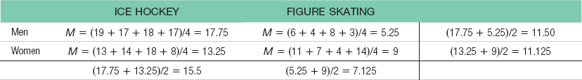
- c. dfrows(gender) = Nrows − 1 = 2 − 1 = 1
dfcolumns(sport) = Ncolumns − 1 = 2 − 1 = 1
dfinteraction = (dfrows)(dfcolumns) = (1)(1) = 1
dfwithin = dfM,H + dfM,S + dfW,H + dfW,S = 3 + 3 + 3 + 3 = 12
dftotal = Ntotal − 1 = 16 − 1 = 15
We can also check that this answer is correct by adding all of the other degrees of freedom together:
1 + 1 + 1 + 12 + 15
The critical value for an F distribution with 1 and 12 degrees of freedom, at a p level of 0.01, is 9.33. - d. GM = 11.313
SStotal = Σ(X - GM)2 for each score = 475.438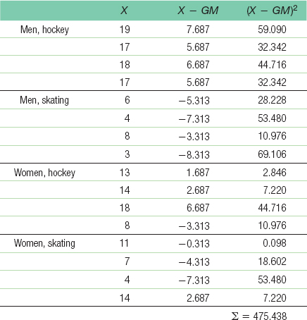
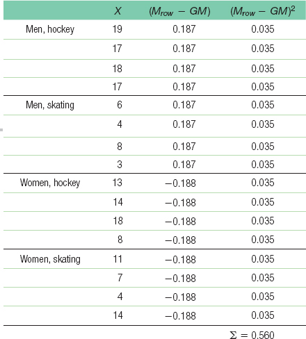
- e. Sum of squares for gender: SSbetween(rows) = Σ(Mrow - GM)2 for each score = 0.560
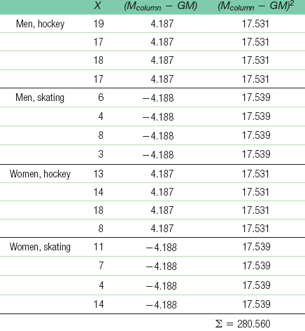
- f. Sum of squares for sporting event: SSbetween(columns) = Σ(Mcolumn − GM)2 for each score = 280.560
C-
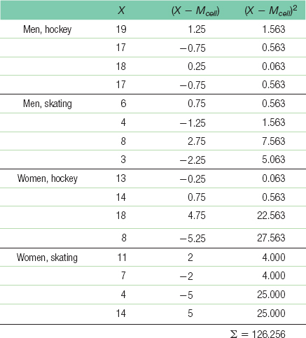
47 - g. SSwithin = Σ(X − Mcell)2 for each score = 126.256
- h. We use subtraction to find the sum of squares for the interaction. We subtract all other sources from the total sum of squares, and the remaining amount is the sum of squares for the interaction.
SSgender × sport = SStotal − (SSgender + SSsport + SSwithin)
SSgender × sport = 475.438 − (0.560 + 280.560 + 126.256) = 68.062 - i.
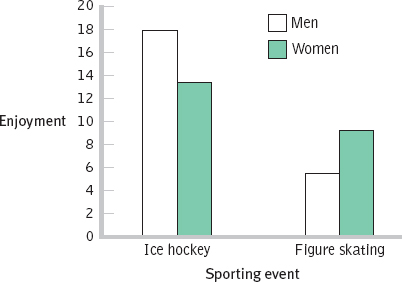
SOURCE SS df MS F Gender 0.560 1 0.560 0.05 Sporting event 280.560 1 280.560 26.67 Gender × sport 68.062 1 68.062 6.47 Within 126.256 12 10.521 Total 475.438 15
- a.
- 14.27
SOURCE SS df MS F Gender 248.25 1 248.25 8.07 Parenting style 84.34 3 28.113 0.91 Gender × style 33.60 3 11.20 0.36 Within 1107.2 36 30.756 Total 1473.39 43 - 14.29 For the main effect A:
According to Cohen’s conventions, this is approaching a medium effect size.
For the main effect B:
According to Cohen’s conventions, this is approaching a medium effect size.
For the interaction: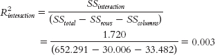
According to Cohen’s conventions, this is smaller than a small effect size. - 14.31
- a. This study would be analyzed with a between-
groups ANOVA because different groups of participants were assigned to the different treatment conditions. - b. This study could be redesigned to use a within-
groups ANOVA by testing the same group of participants on some myths repeated once and some repeated three times both when they are young and then again when they are old.
- a. This study would be analyzed with a between-
- 14.33
- a. There are two independent variables. The first is gender, and its levels are male and female. The second is the gender of the person being sought, and its levels are same-
sex and opposite- sex. - b. The dependent variable is the preferred maximum age difference.
- c. He would use a two-
way between- groups ANOVA. - d. He would use a 2 × 2 between-
groups ANOVA. - e. The ANOVA would have four cells. This number is obtained by multiplying the number of levels of each independent variable (2 × 2).
C-
48 - f.
MALE FEMALE Same- sex Same- sex; male Same- sex; female Opposite- sex Opposite- sex; male Opposite- sex; female
- a. There are two independent variables. The first is gender, and its levels are male and female. The second is the gender of the person being sought, and its levels are same-
- 14.35
- a. The first independent variable is the gender said to be most affected by the illness, and its levels are men and women. The second independent variable is the gender of the participant, and its levels are male and female. The dependent variable is level of comfort, on a scale of 1–
7. - b. The researchers conducted a two-
way between- groups ANOVA. - c. The reported statistics do indicate that there is a significant interaction because the probability associated with the F statistic for the interaction is less than 0.05.
- d.
FEMALE PARTICIPANTS MALE PARTICIPANTS Illness affects woman 4.88 3.29 Illness affects men 3.56 4.67 - e. Bar graph for the interaction:
- f. This is a qualitative interaction. Female participants indicated greater average comfort about attending a meeting regarding an illness that affects women than about attending a meeting regarding an illness that affects men. Male participants had the opposite pattern of results; male participants indicated greater average comfort about attending a meeting regarding an illness that affects men as opposed to one that affects women.
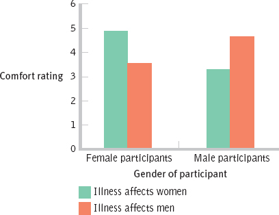
- g.Note: There are several cell means that would work.
FEMALE PARTICIPANTS MALE PARTICIPANTS Illness affects woman 4.88 4.80 Illness affects men 3.56 4.67 - h. Bar graph for the new means:
- i.
FEMALE PARTICIPANTS MALE PARTICIPANTS Illness affects woman 4.88 5.99 Illness affects men 3.56 4.67
- a. The first independent variable is the gender said to be most affected by the illness, and its levels are men and women. The second independent variable is the gender of the participant, and its levels are male and female. The dependent variable is level of comfort, on a scale of 1–
- 14.37
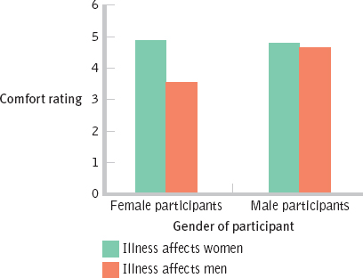
- a. The first independent variable is the race of the face, and its levels are white and black. The second independent variable is the type of instruction given to the participants, and its levels are no instruction and instruction to attend to distinguishing features. The dependent variable is the measure of recognition accuracy.
- b. The researchers conducted a two-
way between- groups ANOVA. - c. The reported statistics indicate that there is a significant main effect of race. On average, the white participants who saw white faces had higher recognition scores than did white participants who saw black faces.
- d. The main effect is misleading because those who received instructions to attend to distinguishing features actually had lower mean recognition scores for the white faces than did those who received no instruction, whereas those who received instructions to attend to distinguishing features had higher mean recognition scores for the black faces than did those who received no instruction.
- e. The reported statistics do indicate that there is a significant interaction because the probability associated with the F statistic for the interaction is less than 0.05.
- f.
BLACK FACE WHITE FACE No instruction 1.04 1.46 Distinguishing features instruction 1.23 1.38 C-
49 - g. Bar graph of findings:
- h. When given instructions to pay attention to distinguishing features of the faces, participants’ average recognition of the black faces was higher than when given no instructions, whereas their average recognition of the white faces was worse than when given no instruction. This is a qualitative interaction because the direction of the effect changes between black and white.
- 14.39
- a. The first independent variable is gender of the seeker, and its levels are men and women. The second independent variable is gender of the person being sought, and its levels are men and women. The dependent variable is the oldest acceptable age of the person being sought.
- b.
WOMEN SEEKERS MEN SEEKERS Men sought 34.80 35.40 Women sought 36.00 27.20 - c. Step 1: Population 1 (women, men) is women seeking men. Population 2 (men, women) is men seeking women. Population 3 (women, women) is women seeking women. Population 4 (men, men) is men seeking men. The comparison distributions will be F distributions. The hypothesis test will be a two-
way between- groups ANOVA.
Assumptions: The data are not from random samples, so we must generalize with caution. The assumption of homogeneity of variance is violated because the largest variance (29.998) is much larger than the smallest variance (1.188). For the purposes of this exercise, however, we will conduct this ANOVA.
Step 2: Main effect of first independent variable—gender of seeker:
Null hypothesis: On average, men and women report the same oldest acceptable ages for a partner—μM = μW.
Research hypothesis: On average, men and women report different oldest acceptable ages for a partner—μM ≠ μW.
Main effect of second independent variable—gender of person sought:
Null hypothesis: On average, those seeking men and those seeking women report the same oldest acceptable ages for a partner—μM = μW
Research hypothesis: On average, those seeking men and those seeking women report different oldest acceptable ages for a partner—μM ≠ μW.
Interaction: Seeker × sought:
Null hypothesis: The effect of the gender of the seeker does not depend on the gender of the person sought. Research hypothesis: The effect of the gender of the seeker does depend on the gender of the person sought.
Step 3: dfcolumns(seeker) = 2 − 1 = 1
dfrows(sought) = 2 − 1 = 1
dfinteraction = (1)(1) = 1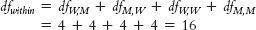
Main effect of gender of seeker: F distribution with 1 and 16 degrees of freedom
Main effect of gender of sought: F distribution with 1 and 16 degrees of freedom
Interaction of seeker and sought: F distribution with 1 and 16 degrees of freedom
Step 4: Cutoff F for main effect of seeker: 4.49
Cutoff F for main effect of sought: 4.49
Cutoff F for interaction of seeker and sought: 4.49
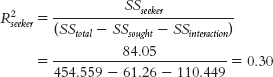
Step 5: SStotal = Σ(X − GM)2 = 454.559
SScolumn(seeker) = Σ(Mcolumn(seeker) − GM)2 = 84.050
SSrow(sought) = Σ(Mrow(sought) + GM)2 = 61.260
SSwithin = Σ(X + Mcell)2 = 198.800
SSinteraction = SStotal − (SSrow + SScolumn + SSwithin) = 110.449Step 6: There is a significant main effect of gender of the seeker; it appears that women are willing to accept older dating partners, on average, than are men. There is also a significant main effect of gender of the person being sought; it appears that those seeking men are willing to accept older dating partners, on average, than are those seeking women. Additionally, there is a significant interaction between the gender of the seeker and the gender of the person being sought. Because there is a significant interaction, we ignore the main effects and report only the interaction.SOURCE SS df MS F Seeker gender 84.050 1 84.050 6.76 Sought gender 61.260 1 61.260 4.93 Seeker × sought 110.449 1 110.449 8.89 Within 198.800 16 12.425 Total 454.559 19 - d. There is a significant quantitative interaction because there is a difference for male seekers, but not for female seekers. We are not seeing a reversal of direction necessary for a qualitative interaction.
C-
50 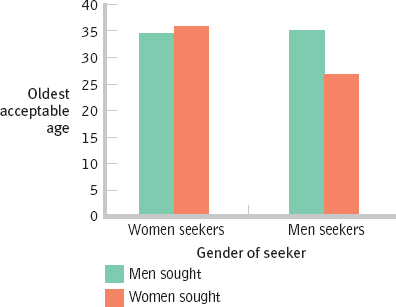
- e. For the main effect of seeker gender:
According to Cohen’s conventions, this is a large effect size.
For the main effect of sought gender: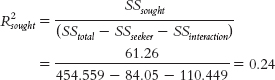
According to Cohen’s conventions, this is a large effect size.
For the interaction: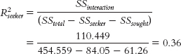
According to Cohen’s conventions, this is a large effect size.
- 14.41
- a. The independent variables are type of payment, still with two levels, and level of payment, now with three levels (low, moderate, and high). The dependent variable is still willingness to help, as assessed with the 11-
point scale. - b.
LOW AMOUNT MODERATE AMOUNT HIGH AMOUNT Cash payment 4.75 7.50 8.00 6.75 Candy payment 6.25 6.00 6.50 6.25 5.50 6.75 7.25 - c.
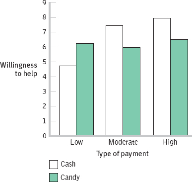
- d. There does still seem to be the same qualitative interaction, such that the effect of the level of payment depends on the type of payment. When candy payments are used, the level seems to have no mean impact. However, when cash payments are used, a low level leads to a lower willingness to help, on average, than when candy is used, and a moderate or high level leads to a higher willingness to help, on average, than when candy is used.
- e. Post hoc tests would be needed. Specifically, we would need to compare the three levels of payment to see where specific significant differences exist. Based on the graph we created, it appears as if willingness to help in the low payment condition is significantly lower, on average, than in the moderate and high conditions for payments.
- a. The independent variables are type of payment, still with two levels, and level of payment, now with three levels (low, moderate, and high). The dependent variable is still willingness to help, as assessed with the 11-
- 14.43
- a. This is problematic because it suggests a causal relation for correlational data. There are many possible confounds. It could be that people with high energy are more likely both to exercise (and lose weight) and to work long hours (and make more money). It could be that education level is associated with both weight and income. The act of losing weight might not cause one’s income to change at all.
- b. If you can include covariates, you can eliminate alternative explanations. There are several possible scale variables that could be included as covariates. For example, if you include education level as a covariate and there is still a link between weight and income, you can eliminate education level as a possible confound.
- 14.45
- a. The independent variables are educational attainment (levels: transitioning adolescents, college underclassmen, college upperclassmen), disability status (levels: dyslexia, ADHD, ADHD/dyslexia), and gender (levels: male, female).
- b. The dependent variables are depression as assessed by the BDI-
II and anxiety as assessed by the BAI. - c. The researchers conducted a MANOVA because multiple dependent variables were being analyzed at the same time.
- d.
- i. Upperclassmen with disabilities have higher levels of depression and anxiety, on average, than do transitioning adolescents with disabilities.
C-
51 - ii. A Tukey HSD test was likely conducted because a statistically significant effect was found for the main effect of educational attainment. Because there were three levels, the researchers would not have known from this statistically significant effect which pairs of the three means were statistically significantly different from each other. The Tukey HSD test allowed the researchers to test each pair of educational attainment levels for mean differences in anxiety and for mean differences in depression.
- iii. Usually the appropriate effect size with ANOVA and its various forms, including MANOVA, is R2. However, in this case, the researchers reported Cohen’s d because the Tukey HSD tests assess the difference between pairs of means, and Cohen’s d reports the differences in terms of standard deviation between pairs of means.
- i. Upperclassmen with disabilities have higher levels of depression and anxiety, on average, than do transitioning adolescents with disabilities.
- 14.47
- a. The independent variables are type of feedback (levels: positive, negative), level of expertise (levels: novice, expert), and domain (level: feedback on language acquisition, pursuit of environmental causes, use of consumer products).
- b. The dependent variable appears to be interest in instructor, seeking behavior, and response behavior.
- c. This interaction is statistically significant, as the p value is less than 0.05.
- d. The statistic missing from this report is a measure of effect size, such as R2. The effect sizes helps us figure out whether something that is statistically significant is also practically important.
- e. The bar graph illustrates what appears to be a qualitative interaction. Experts sought and responded more to negative feedback than to positive feedback; novices sought and responded more to positive feedback than to negative feedback.
- f. Suggestions may vary. The graph needs a clear, specific title; the y-axis should go down to 0; and the label on the y-axis should be rotated so that it reads left to right.