Chapter 15
- 15.1 A correlation coefficient is a statistic that quantifies the relation between two variables.
- 15.3 A perfect relation occurs when the data points fall exactly on the line we fit through the data. A perfect relation results in a correlation coefficient of −1.0 or 1.0.
- 15.5 According to Cohen (1988), a correlation coefficient of 0.50 is a large correlation, and 0.30 is a medium one. However, it is unusual in social science research to have a correlation as high as 0.50. The decision of whether a correlation is worth talking about is sometimes based on whether it is statistically significant, as well as what practical effect a correlation of a certain size indicates.
- 15.7 When used to capture the relation between two variables, the correlation coefficient is a descriptive statistic. When used to draw conclusions about the greater population, such as with hypothesis testing, the coefficient serves as an inferential statistic.
- 15.9 Positive products of deviations, indicating a positive correlation, occur when both members of a pair of scores tend to result in a positive deviation or when both members tend to result in a negative deviation. Negative products of deviations, indicating a negative correlation, occur when members of a pair of scores tend to result in opposite-
valued deviations (one negative and the other positive). - 15.11(1) We calculate the deviation of each score from its mean, multiply the two deviations for each participant, and sum the products of the deviations. (2) We calculate a sum of squares for each variable, multiply the two sums of squares, and take the square root of the product of the sums of squares. (3) We divide the sum from step 1 by the square root in step 2.
- 15.13 Test—
retest reliability involves giving the same group of people the exact same test with some amount of time (perhaps a week) between the two administrations of the test. Test— retest reliability is then calculated as the correlation between their scores on the two administrations of the test. Calculation of coefficient alpha does not require giving the same test two times. Rather, coefficient alpha is based on correlations between different halves of the test items from a single administration of the test. - 15.15 The difference between a Pearson correlation coefficient and a partial correlation coefficient is that the partial correlation coefficient has factored out the influence of one or more additional variables; thus, it is a better representation of the relation between the two variables because it controls for other related variables.
- 15.17
- a. These data appear to be negatively correlated.
- b. These data appear to be positively correlated.
- c. Neither; these data appear to have a very small correlation, if any.
- 15.19
- a. −0.28 is a medium correlation.
- b. 0.79 is a large correlation.
- c. 1.0 is a perfect correlation.
- d. −0.015 is almost no correlation.
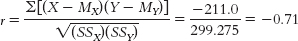
- 15.21
- a.
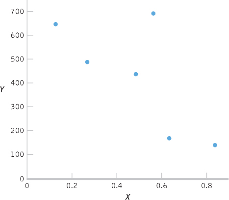
C-
52 - b.
X (X − MX) Y (Y − MY) (X − MX) (Y − MY) 0.13 −0.36 645 218.50 −78.660 0.27 −0.22 486 59.50 −13.090 0.49 0.00 435 8.50 0.000 0.57 0.08 689 262.50 21.000 0.84 0.35 137 −289.50 −101.325 0.64 0.15 167 −259.50 −38.925 MX = 0.49 MY = 426.5 Σ[(X − MX)(Y − MY)] = −211.0 - c.
X (X − MX) (X − MX)2 Y (Y − MY) (Y − MY)2 0.13 −0.36 0.130 645 218.50 47,742.25 0.27 −0.22 0.048 486 59.50 3540.25 0.49 0.00 0.000 435 8.50 72.25 0.57 0.08 0.006 689 262.50 68,906.25 0.84 0.35 0.123 137 −289.50 83,810.25 0.64 0.15 0.023 167 −259.50 67,340.25 Σ(X − MX)2 = 0.330 Σ (Y − MY)2 = 271,411.50 
- d.
- e. dfr = N − 2 = 6 − 2 = 4
- f. −0.811 and 0.811
- a.
- 15.23
- a.
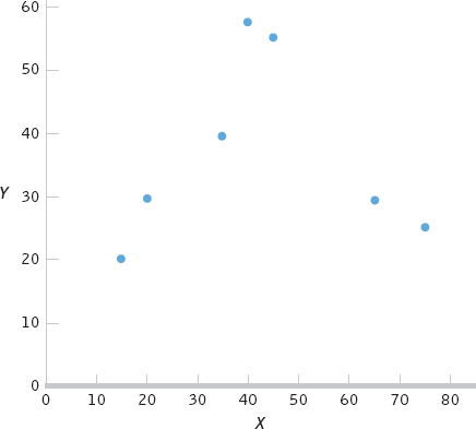
- b.
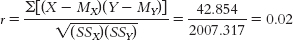
X (X − MX) Y (Y − MY) (X − MX) (Y − MY) 40 −2.143 60 22.857 −48.983 45 2.857 55 17.857 51.017 20 −22.143 30 −7.143 158.167 75 32.857 25 −12.143 −398.983 15 −27.143 20 −17.143 465.312 35 −7.143 40 2.857 −20.408 65 22.857 30 −7.143 163.268 MX = 42.143 MY = 37.143 Σ[(X − MX)(Y − MY)] = 42.854 - c.
X (X − MX) (X − MX)2 Y (Y − MY) (Y − MY)2 40 −2.143 4.592 60 22.857 522.442 45 2.857 8.162 55 17.857 318.872 20 −22.143 490.312 30 −7.143 51.022 75 32.857 1079.582 25 −12.143 147.452 15 −27.143 736.742 20 −17.143 293.882 35 −7.143 51.022 40 2.857 8.162 65 22.857 522.442 30 −7.143 51.022 Σ(X − MX)2 = 2892.854 Σ(Y − MY)2 = 1392.854 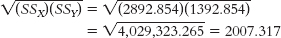
- d.
- e. dfr = N − 2 = 7 − 2 = 5
- f. −0.754 and 0.754
- a.
- 15.25
- a. dfr = N − 2 = 3113 − 2 = 3111. The highest degrees of freedom listed on the table is 100, with cutoffs of −0.195 and 0.195.
- b. dfr = N − 2 = 72 − 2 = 70; −0.232 and 0.232
- 15.27 When using a measure to diagnose individuals, having a reliability of at least 0.90 is important—
and the more reliable the test, the better. So, based on reliability information alone, we would recommend she use the test with 0.95 reliability. - 15.29 The third variable does not account for any of the correlation between A and B. The partial correlation, taking into account the third variable, is exactly the same as the original correlation between A and B.
- 15.31
- a. Newman’s data do not suggest a correlation between Mercury’s phases and breakdowns. There was no consistency in the report of breakdowns during one of the phases.
- b. Massey may observe a correlation because she already believes that there is a relation between astrological events and human events. As you learned in Chapter 5, the confirmation bias refers to the tendency to pay attention to those events that confirm our prior beliefs. The confirmation bias may lead Massey to observe an illusory correlation (i.e., she perceives a correlation that does not actually exist) because she attends only to those events that confirm her prior belief that the phase of Mercury is related to breakdowns.
C-
53 - c. Given that there are two phases of Mercury (and assuming they’re equal in length), half of the breakdowns that occur would be expected to occur during the retrograde phase and the other half during the nonretrograde phase, just by chance. Expected relative-
frequency probability refers to the expected frequency of events. So in this example we would expect 50% of breakdowns to occur during the retrograde phase and 50% during the nonretrograde phase. If we base our conclusions on only a small number of observations of breakdowns, the observed relative- frequency probability is more likely to differ from the expected relative- frequency probability because we are less likely to have a representative sample of breakdowns. - d. This correlation would not be useful in predicting events in your own life because no relation would be observed in this limited time span.
- e. Available data do not support the idea that a correlation exists between Mercury’s phases and breakdowns.
- 15.33
- a. The accompanying scatterplot depicts the relation between hours of exercise and number of friends. Note that you could have chosen to put hours of exercise along the y-axis and number of friends along the x-axis.
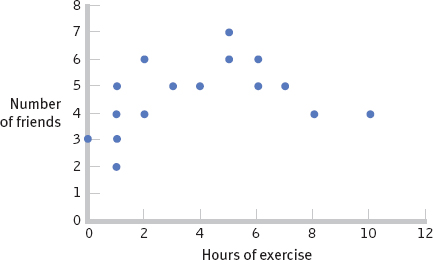
- b. The scatterplot suggests that as the number of hours of exercise each week increases from 0 to 5, there is an increase in the number of friends, but as the hours of exercise continue to increase past 5, there is a decrease in the number of friends.
- c. It would not be appropriate to calculate a Pearson correlation coefficient with this set of data. The scatterplot suggests a nonlinear relation between exercise and number of friends, and the Pearson correlation coefficient measures only the extent of linear relation between two variables.
- a. The accompanying scatterplot depicts the relation between hours of exercise and number of friends. Note that you could have chosen to put hours of exercise along the y-axis and number of friends along the x-axis.
- 15.35Step 1: Population 1: Adolescents like those we studied. Population 2: Adolescents for whom there is no relation between externalizing behavior and anxiety. The comparison distribution is made up of correlation coefficients based on many, many samples of our size, 10 people, randomly selected from the population.
We do not know if the data were randomly selected (first assumption), so we must be cautious when generalizing the findings. We also do not know if the underlying population distribution for externalizing behaviors and anxiety in adolescents is normally distributed (second assumption). The sample size is too small to make any conclusions about this assumption, so we should proceed with caution. The third assumption, unique to correlation, is that the variability of one variable is equal across the levels of the other variable. Because we have such a small data set, it is difficult to evaluate this. However, we can see from the scatterplot that the data are somewhat consistently variable.
Step 2: Null hypothesis: There is no correlation between externalizing behavior and anxiety among adolescents—H0: ρ = 0.
Research hypothesis: There is a correlation between externalizing behavior and anxiety among adolescents—H1: ρ ≠ 0.
Step 3: The comparison distribution is a distribution of Pearson correlations, r, with the following degrees of freedom: dfr = N − 2 = 10 − 2 = 8.
Step 4: The critical values for an r distribution with 8 degrees of freedom for a two-tailed test with a p level of 0.05 are −0.632 and 0.632.
Step 5: The Pearson correlation coefficient is calculated in three steps. First, we calculate the numerator:Second, we calculate the denominator:X (X − MX) Y (Y − MY) (X − MX) (Y − MY) 9 2.40 37 7.60 18.24 7 0.40 23 −6.40 −2.56 7 0.40 26 −3.40 −1.36 3 −3.60 21 −8.40 30.24 11 4.40 42 12.60 55.44 6 −0.60 33 3.60 −2.16 2 −4.60 26 −3.40 15.64 6 −0.60 35 5.60 −3.36 6 −0.60 23 −6.40 3.84 9 2.40 28 −1.40 −3.36 MX = 6.60 MY = 29.40 Σ[(X − MX)(Y − MY)] = 110.60 X (X − MX) (X − MX)2 Y (Y − MY) (Y − MY)2 9 2.40 5.76 37 7.60 57.76 7 0.40 0.16 23 −6.40 40.96 7 0.40 0.16 26 −3.40 11.56 3 −3.60 12.96 21 −8.40 70.56 11 4.40 19.36 42 12.60 158.76 6 −0.60 0.36 33 3.60 12.96 2 −4.60 21.16 26 −3.40 11.56 6 −0.60 0.36 35 5.60 31.36 6 −0.60 0.36 23 −6.40 40.96 9 2.40 5.76 28 −1.40 1.96 Σ(X − MX)2 = 66.40 Σ(Y − MY)2 = 438.40 
Finally, we compute r: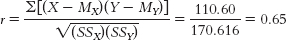 The test statistic, r = 0.65, is larger in magnitude than the critical value of 0.632. We can reject the null hypothesis and conclude that there is a strong positive correlation between the number of externalizing behaviors performed by adolescents and their level of anxiety.
C-
54 - 15.37
- a. You might expect a person who owns a lot of cats to tend to have many mental health problems. Because the two variables are positively correlated, as cat ownership increases, the number of mental health problems tends to increase.
- b. You might expect a person who owns no cats or just one cat to tend to have few mental health problems. Because the variables are positively correlated, people who have a low score on one variable are also likely to have a low score on the other variable.
- c. You might expect a person who owns a lot of cats to tend to have few mental health problems. Because the two variables are negatively related, as one variable increases, the other variable tends to decrease. This means a person owning lots of cats would likely have a low score on the mental health variable.
- d. You might expect a person who owns no cats or just one cat to tend to have many mental health problems. Because the two variables are negatively related, as one variable decreases, the other variable tends to increase, which means that a person with fewer cats would likely have more mental health problems.
- 15.39
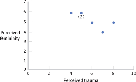
- a. The accompanying scatterplot depicts a negative linear relation between perceived femininity and perceived trauma. Because the relation appears linear, it is appropriate to calculate the Pearson correlation coefficient for these data. (Note: The number (2) indicates that two participants share that pair of scores.)
- b. The Pearson correlation coefficient is calculated in three steps. Step 1 is calculating the numerator:Step 2 is calculating the denominator:
X (X − MX) Y (Y − MY) (X − MX)(Y − MY) 5 −0.833 6 0.667 −0.556 6 0.167 5 −0.333 −0.056 4 −1.833 6 0.667 −1.223 5 −0.833 6 0.667 −0.556 7 1.167 4 −1.333 −1.556 8 2.167 5 −0.333 −0.722 MX = 5.833 MY = 5.333 Σ[(X − MX)(Y − MY)] = −4.669 X (X − MX) (X − MX)2 Y (Y − MY) (Y − MY)2 5 −0.833 0.694 6 0.667 0.445 6 0.167 0.028 5 −0.333 0.111 4 −1.833 3.360 6 0.667 0.445 5 −0.833 0.694 6 0.667 0.445 7 1.167 1.362 4 −1.333 1.777 8 2.167 4.696 5 −0.333 0.111 Σ[(X − MX)2 = 10.834 Σ(Y − MY)2 = 3.334 
Step 3 is computing r: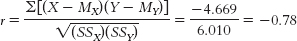
- c. The correlation coefficient reveals a strong negative relation between perceived femininity and perceived trauma; as trauma increases, perceived femininity tends to decrease.
- d. Those participants who had positive deviation scores on trauma tended to have negative deviation scores on femininity (and vice versa), meaning that when a person’s score on one variable was above the mean for that variable (positive deviation), his or her score on the second variable was typically below the mean for that variable (negative deviation). So, having a high score on one variable was associated with having a low score on the other, which is a negative correlation.
- a. The accompanying scatterplot depicts a negative linear relation between perceived femininity and perceived trauma. Because the relation appears linear, it is appropriate to calculate the Pearson correlation coefficient for these data. (Note: The number (2) indicates that two participants share that pair of scores.)
- 15.41
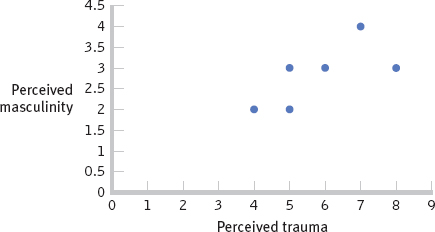
- a. The scatterplot on the next page depicts a positive linear relation between perceived trauma and perceived masculinity. The data appear to be linearly related; therefore, it is appropriate to calculate a Pearson correlation coefficient.
- b. The Pearson correlation coefficient is calculated in three steps. Step 1 is calculating the numerator:
X (X − MX) Y (Y − MY) (X − MX)(Y − MY) 5 −0.833 3 0.167 −0.139 6 0.167 3 0.167 0.028 4 −1.833 2 −0.833 1.527 5 −0.833 2 −0.833 0.694 7 1.167 4 1.167 1.362 8 2.167 3 0.167 0.362 MX = 5.833 MY = 2.833 Σ[(X − MX)(Y − MY)] = 3.834 Step 2 is calculating the denominator:C-
55 X (X − MX) (X − MX)2 Y (Y − MY) (Y − MY)2 5 −0.833 0.694 3 0.167 0.028 6 0.167 0.028 3 0.167 0.028 4 −1.833 3.360 2 −0.833 0.694 5 −0.833 0.694 2 −0.833 0.694 7 1.167 1.362 4 1.167 1.362 8 2.167 4.696 3 0.167 0.028 Σ[(X − MX)2 = 10.834 Σ(Y − MY)2 = 2.834 
Step 3 is computing r: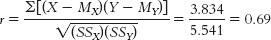
- c. The correlation coefficient is large and positive. This means that as ratings of trauma increased, ratings of masculinity tended to increase as well.
- d. For most of the participants, the sign of the deviation for the traumatic variable is the same as that for the masculinity variable, which indicates that those participants scoring above the mean on one variable also tended to score above the mean on the second variable (and likewise for the lowest scores). Because the scores for each participant tend to fall on the same side of the mean, this is a positive relation.
- e. When the soldier was a woman, the perception of the situation as traumatic was strongly negatively correlated with the perception of the woman as feminine. This relation is opposite that observed when the soldier was a man. When the soldier was a man, the perception of the situation as traumatic was strongly positively correlated with the perception of the man as feminine. Regardless of whether the soldier was a man or a woman, there was a positive correlation between the perception of the situation as traumatic and the perception of masculinity, but the observed correlation was stronger for the perceptions of women than for the perceptions of men.
- a. The scatterplot on the next page depicts a positive linear relation between perceived trauma and perceived masculinity. The data appear to be linearly related; therefore, it is appropriate to calculate a Pearson correlation coefficient.
- 15.43
- a. Because your friend is running late, she is likely more concerned about traffic than she otherwise would be. Thus, she may take note of traffic only when she is running late, leading her to believe that the amount of traffic correlates with how late she is. Furthermore, having this belief, in the future she may think only of cases that confirm her belief that a relation exists between how late she is and traffic conditions, reflecting a confirmation bias. Alternatively, traffic conditions might be worse when your friend is running late, but that could be a coincidence. A more systematic study of the relation between your friend’s behavior and traffic conditions would be required before she could conclude that a relation exists.
- b. There are a number of possible answers to this question. For example, we could operationalize the degree to which she is late as the number of minutes past her intended departure time that she gets in the car. We could operationalize the amount of traffic as the number of minutes the car is being driven at less than the speed limit (given that your friend would normally drive right at the speed limit).
- 15.45
- a. The reporter suggests that convertibles are not generally less safe than other cars.
- b. Convertibles may be driven less often than other cars, as they may be considered primarily a recreational vehicle. If they are driven less, owners have fewer chances to get into accidents while driving them.
- c. A more appropriate comparison may be to determine the number of fatalities that occur per every 100 hours driven in various kinds of cars.
- 15.47
- a. The researchers are suggesting that participation in arts education programs causes students to tend to perform better and stay in school longer.
- b. It could be that those students who perform better and stay in school longer are more likely to be interested in, and therefore participate in, arts education programs.
- c. There are many possible answers. For example, the socioeconomic status of the students’ families may be associated with performance in school, years of schooling, and participation in arts education programs, with higher socioeconomic status tending to lead to improved performance, staying in school longer, and higher participation in arts education programs.
- 15.49
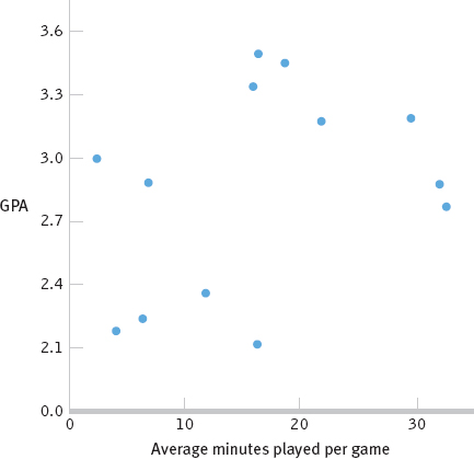
- a. It appears that the data are somewhat positively correlated.
- b. The Pearson correlation coefficient is calculated in three steps. Step 1 is calculating the numerator:
X (X − MX) Y (Y − MY) (X − MX) (Y − MY) 29.70 13.159 3.20 0.343 4.514 32.14 15.599 2.88 0.023 0.359 32.72 16.179 2.78 −0.077 −1.246 21.76 5.219 3.18 0.323 1.686 18.56 2.019 3.46 0.603 1.217 16.23 −0.311 2.12 −0.737 0.229 11.80 −4.741 2.36 −0.497 2.356 6.88 −9.661 2.89 0.033 −0.319 6.38 −10.161 2.24 −0.617 6.269 15.83 −0.711 3.35 0.493 −0.351 2.50 −14.041 3.00 0.143 −2.008 4.17 −12.371 2.18 −0.677 8.375 16.36 −0.181 3.50 0.643 −0.116 MX = 16.541 MY = 2.857 Σ[(X − MX)(Y − MY)] = 20.965 Step 2 is calculating the denominator:C-
56 X (X − MX) (X − MX)2 Y (Y − MY) (Y − MY)2 29.70 13.159 173.159 3.20 0.343 0.118 32.14 15.599 243.329 2.88 0.023 0.001 32.72 16.179 261.760 2.78 −0.077 0.006 21.76 5.219 27.238 3.18 0.323 0.104 18.56 2.019 4.076 3.46 0.603 0.364 16.23 −0.311 0.097 2.12 −0.737 0.543 11.80 −4.741 22.477 2.36 −0.497 0.247 6.88 −9.661 93.335 2.89 0.033 0.001 6.38 −10.161 103.246 2.24 −0.617 0.381 15.83 −0.711 0.506 3.35 0.493 0.243 2.50 −14.041 197.150 3.00 0.143 0.020 4.17 −12.371 153.042 2.18 −0.677 0.458 16.36 −0.181 0.033 3.50 0.643 0.413 Σ(X − MX)2 = 1279.448 Σ(Y − MY)2 = 2.899 
Step 3 is computing r: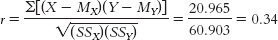
- c. We computed the correlation coefficient for these data to explore whether there was a relation between GPA and playing time for the members of this team. If we were interested in making a statement about athletes in general, an inferential analysis, we would want to collect more data from a random or representative sample and conduct a hypothesis test.
- d. Step 1: Population 1: Athletes like those we studied. Population 2: Athletes for whom there is no relation between minutes played and GPA. The comparison distribution is made up of many, many correlation coefficients based on samples of our size, 13 people, randomly selected from the population.
We know that these data were not randomly selected (first assumption), so we must be cautious when generalizing the findings. We also do not know if the underlying population distributions are normally distributed (second assumption). The sample size is too small to make any conclusions about this assumption, so we should proceed with caution. The third assumption, unique to correlation, is that the variability of one variable is equal across the levels of the other variable. Because we have such a small data set, it is difficult to evaluate this.
Step 2: Null hypothesis: There is no correlation between participation in athletics, as measured by minutes played on average, and GPA—H0: ρ = 0.
Research hypothesis: There is a correlation between participation in athletics and GPA—H1: ρ ≠ 0.
Step 3: The comparison distribution is a distribution of Pearson correlation coefficients, r, with the following degrees of freedom: dfr = N − 2 = 13 − 2 = 11.
Step 4: The critical values for an r distribution with 11 degrees of freedom for a two-tailed test with a p level of 0.05 are −0.553 and 0.553.
Step 5: r = 0.34, as calculated in b.
Step 6: The test statistic, r = 0.34, is not larger in magnitude than the critical value of 0.553, so we fail to reject the null hypothesis. We cannot conclude that a relation exists between these two variables. Because the sample size is rather small and we calculated a medium correlation with this small sample, we would be encouraged to collect more data to increase statistical power so that we may more fully explore this relation. - e. Because the results are not statistically significant, we cannot draw any conclusion, except that we do not have enough information.
- f. We could have collected these data randomly, rather than looking at just one team. We also could have collected a larger sample size. In order to say something about causation, we could manipulate average minutes played to see whether that manipulation results in a change in GPA. Because very few coaches would be willing to let us do that, we would have a difficult time conducting such an experiment.
- a. It appears that the data are somewhat positively correlated.
- 15.51
- a. If students were marked down for talking about the rooster rather than the cow, the reading test would not meet the established criteria. The question asked on the test is ambiguous because the information regarding what caused the cow’s behavior to change is not explicitly stated in the story. Furthermore, the correct answer to the question provided on the Web site is not actually an answer to the question itself. The question states, “What caused Brownie’s behavior to change?” The answer that the cow started out kind and ended up mean is a description of how her behavior changed, not what caused her behavior to change. This question does not appear to be a valid question because it does not appear to provide an accurate assessment of students’ writing ability.
- b. One possible third variable that could lead to better performance in some schools over others is the average socioeconomic status of the families whose children attend the school. Schools in wealthier areas or counties would have students of higher socioeconomic status, who might be expected to perform better on a test of writing skill. A second possible third variable that could lead to better performance in some schools over others is the type of reading and writing curriculum implemented in the school. Different ways of teaching the material may be more effective than others, regardless of the effectiveness of the teachers who are actually presenting the material.
- 15.53
- a. The participants in the study are the various countries on which rates were obtained.
- b. The two variables are health care spending and health, as assessed by life expectancy. Health care spending was operationalized as the amount spent per capita on health care, whereas life expectancy is the average age at death. Another way to operationalize health could be rates of various diseases, such as heart disease, or obesity via body mass index (BMI).
C-
57 - c. The study finding was that there is a negative correlation between health care spending and life expectancy, in which countries, such as the United States, that have higher rates of spending on health care per capita have lower life expectancies. One would suspect the opposite to be true, that the more a country spends on health care, the healthier the population would be, thus resulting in higher life expectancy.
- d. Other possible third variables could be the typical body weight in a country, the typical exercise levels in a country, accident rates, access to health care, access or knowledge of preventative health measures, stereotypes, or a country’s typical diet.
- e. This study is a correlational study, not a true experiment, because countries were not assigned to certain levels of health care spending, and then assessed for life expectancy. The data were obtained from naturally occurring events.
- f. It would not be possible to conduct a true experiment on this topic as this would require a manipulation in the health care spending for various countries for the entire population for a long period of time, which would not be realistic, practical, or ethical to implement.
- 15.55
- a. High school athletic participation might be operationalized as a nominal variable by indicating whether a student participates in athletics (levels: yes or no), or by categorizing each student according to the type of athletics (levels: none, football, baseball, etc.) in which they participate.
- b. High school athletic participation might be operationalized as a scale variable by counting the number of sports in which a student participates (e.g., 0, 1, 2), or by counting the number of days on which a student participates in sports annually.
- c. Correlation is a useful tool to quantify the relation between two scale variables, especially when manipulation of either variable does not or cannot occur, and measuring either variable on a nominal or ordinal level would result in information being lost.
- d. The researchers reported the following positive correlations: high school athletic participation and high school GPA; high school athletic participation and college completion; high school athletic participation and earnings as an adult; and high school athletic participation and various positive health behaviors. There are several other positive correlations among only male students; they include the following: high school athletic performance and alcohol consumption; high school athletic performance and sexist attitudes; high school athletic performance and homophobic attitudes; and high school athletic performance and violence. These are all positive correlations because as high school athletic participation increases, so does each of these variables.
- e. There are no negative correlations reported; in all cases, an increase in one variable tended to accompany an increase in the other variable.
- f. One possible causal explanation is that high school athletic participation (A) tends to cause positive health behaviors (B). A second possible causal explanation is that positive health behaviors (B) tend to cause high school athletic participation (A). A third possible causal explanation is that some other variable, such as socioeconomic status (C), could tend to affect both high school athletic participation and positive health behaviors.
- g. Partial correlation might be useful in this study because it would allow us to factor out, or control for, the contribution of a third (or fourth) variable to a relation between two variables. For example, we could calculate the partial correlation between high school athletic participation and college completion, controlling for high school or college GPA.