Chapter 16
- 16.1 Regression allows us to make predictions based on the relation established in the correlation. Regression also allows us to consider the contributions of several variables.
- 16.3 There is no difference between these two terms. They are two ways to express the same thing.
- 16.5a is the intercept, the predicted value for Y when X is equal to 0, which is the point at which the line crosses, or intercepts, the y-axis. b is the slope, the amount that Y is predicted to increase for an increase of 1 in X.
- 16.7 The intercept is not meaningful or useful when it is impossible to observe a value of 0 for X. If height is being used to predict weight, it would not make sense to talk about the weight of someone with no height.
- 16.9 The line of best fit in regression means that we couldn’t make the line a little steeper, or raise or lower it, in any way that would allow it to represent those dots any better than it already does. This is why we can look at the scatterplot around this line and observe that the line goes precisely through the middle of the dots. Statistically, this is the line that leads to the least amount of error in prediction.
- 16.11 Data points clustered closely around the line of best fit are described by a small standard error of the estimate; this allows us to have a high level of confidence in the predictive ability of the independent variable. Data points clustered far away from the line of best fit are described by a large standard error of the estimate, and result in our having a low level of confidence in the predictive ability of the independent variable.
- 16.13 If regression to the mean did not occur, every distribution would look bimodal, like a valley. Instead, the end result of the phenomenon of regression to the mean is that things look unimodal, like a hill or what we call the normal, bell-
shaped curve. Remember that the center of the bell- shaped curve is the mean, and this is where the bulk of data cluster, thanks to regression to the mean. - 16.15 The sum of squares total, SStotal, represents the worst-
case scenario, the total error we would have in the predictions if there were no regression equation and we had to predict the mean for everybody. - 16.17(1) Determine the error associated with using the mean as the predictor. (2) Determine the error associated with using the regression equation as the predictor. (3) Subtract the error associated with the regression equation from the error associated with the mean. (4) Divide the difference (calculated in step 3) by the error associated with using the mean.
C-
58 - 16.19 An orthogonal variable is an independent variable that makes a separate and distinct contribution in the prediction of a dependent variable, as compared with the contributions of another independent variable.
- 16.21 Multiple regression is often more useful than simple linear regression because it allows us to take into account the contribution of multiple independent variables, or predictors, and increase the accuracy of prediction of the dependent variable, thus reducing the prediction error. Because behaviors are complex and tend to be influenced by many factors, multiple regression allows us to better predict a given outcome.
- 16.23 Because the computer software determines which independent variable to enter into the regression equation first and because that first independent variable “wins” all of the variance that it shares with the dependent variable, other variables that are highly correlated with both the first independent variable and with the dependent variable may not reach significance in the regression. Therefore, the researcher may not realize the importance of another potential predictor and may get different results when doing the same regression in another sample.
- 16.25 A latent variable is one that cannot be observed or directly measured but is believed to exist and to influence behavior. A manifest variable is one that can be observed and directly measured and that is an indicator of the latent variable.
- 16.27
- a.
- b. zŶ = (rXY)(zX) = (0.31)(1.667) = 0.517
- c. Ŷ = zŶ (SDY) + MY = (0.517)(3.2) + 10 = 11.65
- a.
- 16.29
- a.
- b. zŶ = (rXY)(zX) = (20.19)(1.75) = −0.333
- c. Ŷ = zŶ (SDY) + MY + (−0.333)(95) + 1000 = 968.37
- d. The y intercept occurs when X is equal to 0. We start by finding a z score:
This is the z score for an X of 0. Now we need to figure out the predicted z score on Y for this X value:
zŶ = (rXY)(zX) = (−0.19)(−4.583) = 0.871
The final step is to convert the predicted z score on this predicted Y to a raw score:
Ŷ = zŶ (SDY) + MY = (0.871)(95) + 1000 = 1082.745
This is the y intercept. - e. The slope can be found by comparing the predicted Y value for an X value of 0 (the intercept) and an X value of 1. Using the same steps as in part (a), we can compute the predicted Y score for an X value of 1.
This is the z score for an X of 1. Now we need to figure out the predicted z score on Y for this X value:
zŶ = (rXY)(zX) = (−0.19)(−4.5) = 0.855
The final step is to convert the predicted z score on this predicted Y to a raw score:
Ŷ = zŶ (SDY) + MY = (0.855)(95) + 1000 = 1081.225
We compute the slope by measuring the change in Y with this 1-unit increase in X:
1081.225 − 1082.745 = −1.52
This is the slope. - f. Ŷ = 1082.745 − 1.52(X)
- g. In order to draw the line, we have one more Ŷ value to compute. This time we can use the regression equation to make the prediction:
Ŷ = 1082.745 − 1.52(48) = 1009.785
Now we can draw the regression line.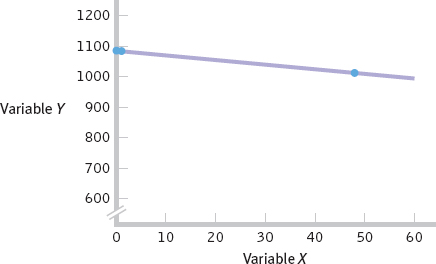
- a.
- 16.31
- a. Ŷ = 49 + (−0.18)(X) = 49 + (−0.18)(−31) = 54.58
- b. Ŷ = 49 + (−0.18)(65) = 37.3
- c. Ŷ = 49 + (−0.18)(14) = 46.48
- 16.33
- a. The sum of squared error for the mean, SStotal:
X Y MY ERROR SQUARED ERROR 4 6 6.75 −0.75 0.563 6 3 6.75 −3.75 14.063 7 7 6.75 0.25 0.063 8 5 6.75 −1.75 3.063 9 4 6.75 −2.75 7.563 10 12 6.75 5.25 27.563 12 9 6.75 2.25 5.063 14 8 6.75 1.25 1.563 SStotal = Σ(Y − MY)2 = 59.504 C-
59 - b. The sum of squared error for the regression equation, SSerror:
X Y REGRESSION EQUATION Y ERROR (Y − Ŷ) SQUARED ERROR 4 6 Ŷ = 2.643 + 0.469(4) = 4.519 1.481 2.193 6 3 Ŷ = 2.643 + 0.469(6) = 5.457 −2.457 6.037 7 7 Ŷ = 2.643 + 0.469(7) = 5.926 1.074 1.153 8 5 Ŷ = 2.643 + 0.469(8) = 6.395 −1.395 1.946 9 4 Ŷ = 2.643 + 0.469(9) = 6.864 −2.864 8.202 10 12 Ŷ = 2.643 + 0.469(10) = 7.333 4.667 21.781 12 9 Ŷ = 2.643 + 0.469(12) = 8.271 0.729 0.531 14 8 Ŷ = 2.643 + 0.469(14) = 9.209 −1.209 1.462 SSerror = Σ(Y − Ŷ)2 = 43.305 - c. The proportionate reduction in error for these data:
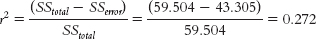
- d. This calculation of r2, 0.272, equals the square of the correlation coefficient, r2 = (0.52)(0.52) = 0.270. These numbers are slightly different due to rounding decisions.
- e. The standardized regression coefficient is equal to the correlation coefficient for simple linear regression, 0.52. We can also check that this is correct by computing β:
X (X − MX) (X − MX)2 Y (Y − MY) (Y − MY)2 4 −4.75 22.563 6 −0.75 0.563 6 −2.75 7.563 3 −3.75 14.063 7 −1.75 3.063 7 0.25 0.063 8 −0.75 0.563 5 −1.75 3.063 9 0.25 0.063 4 −2.75 7.563 10 1.25 1.563 12 5.25 27.563 12 3.25 10.563 9 2.25 5.063 14 5.25 27.563 8 1.25 1.563 Σ(X − MX)2 = 73.504 Σ(Y − MY)2 = 59.504 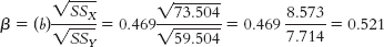
- a. The sum of squared error for the mean, SStotal:
- 16.35
- a.
- b.
- c.
- d.
- a.
- 16.37
- a. The strongest relation depicted in the model is between identity maturity at age 26 and emotional adjustment at age 26. The strength of the path between the two is 0.81.
- b. Positive parenting at age 17 is not directly related to emotional adjustment at age 26 because the two variables are not connected by a link in the model.
- c. Positive parenting at age 17 is directly related to identity maturity at age 26 because the two variables are connected by a direct link in the model.
- d. The variables in boxes are those that were explicitly measured—
the manifest variables. The variables in circles are latent variables— variables that were not explicitly measured but are underlying constructs that the manifest variables are thought to reflect.
- 16.39
- a. Outdoor temperature is the independent variable.
- b. Number of hot chocolates sold is the dependent variable.
- c. As the outdoor temperature increases, we would expect the sale of hot chocolate to decrease.
- d. There are several possible answers to this question. For example, the number of fans in attendance may positively predict the number of hot chocolates sold. The number of children in attendance may also positively predict the number of hot chocolates sold. The number of alternative hot beverage choices may negatively predict the number of hot chocolates sold.
- 16.41
- a. X = z(σ) + μ = −1.2(0.61) + 3.51 = 2.778. This answer makes sense because the raw score of 2.778 is a bit more than 1 standard deviation below the mean of 3.51.
- b. X = z(σ) + μ = 0.66(0.61) + 3.51 = 3.913. This answer makes sense because the raw score of 3.913 is slightly more than 0.5 standard deviation above the mean of 3.51.
- 16.43
- a. 3.12
- b. 3.16
- c. 3.18
C-
60 - d. The accompanying graph depicts the regression line for GPA and hours studied.
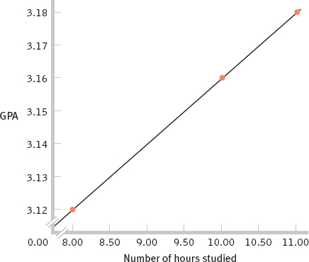
- e. We can calculate the number of hours one would need to study in order to earn a 4.0 by substituting 4.0 for Ŷ in the regression equation and solving for X: 4.0 = 2.96 + 0.02(X). To isolate the X, we subtract 2.96 from the left side of the equation and divide by 0.02: X = (4.0 − 2.96)/0.02 = 52. This regression equation predicts that we would have to study 52 hours a week in order to earn a 4.0. It is misleading to make predictions about what will happen when a person studies this many hours because the regression equation for prediction is based on a sample that studied far fewer hours. Even though the relation between hours studied and GPA was linear within the range of studied scores, outside of that range it may have a different slope or no longer be linear, or the relation may not even exist.
- 16.45
- a. We cannot conclude that cola consumption causes a decrease in bone mineral density because there are a number of different kinds of causal relations that could lead to the predictive relation observed by Tucker and colleagues (2006). There may be some characteristic about these older women that both causes them to drink cola and leads to a decrease in bone mineral density. For example, perhaps overall poorer health habits lead to an increased consumption of cola and a decrease in bone mineral density.
- b. Multiple regression allows us to assess the contributions of more than one independent variable to the outcome, the dependent variable. Performing this multiple regression allowed the researchers to explore the unique contributions of a third variable, such as physical activity, in addition to bone density.
- c. Physical activity might produce an increase in bone mineral density, as exercise is known to increase bone density. Conversely, it is possible that physical activity might produce a decrease in cola consumption because people who exercise more might drink beverages that are more likely to keep them hydrated (such as water or sports drinks).
- d. Calcium intake should produce an increase in bone mineral density, thereby producing a positive relation between calcium intake and bone density. It is possible that consumption of cola means less consumption of beverages with calcium in them, such as milk, producing a negative relation between cola consumption and bone density.
- 16.47
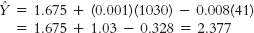
- a. Ŷ = 24.698 + 0.161(X), or predicted year 3 anxiety = 24.698 + 0.161 (year 1 depression)
- b. As depression at year 1 increases by 1 point, predicted anxiety at year 3 increases, on average, by the slope of the regression equation, which is 0.161.
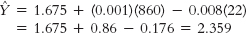
- c. We would predict that her year 3 anxiety score would be 26.31.
- d. We would predict that his year 3 anxiety score would be 25.02.
- 16.49
- a. The independent variable in this study was marital status, and the dependent variable was chance of breaking up.
- b. It appears the researchers initially conducted a simple linear regression and then conducted a multiple regression analysis to account for the other variables (e.g., age, financial status) that may have been confounded with marital status in predicting the dependent variable.
- c. Answers will differ, but the focus should be on the statistically significant contribution these other variables had in predicting the dependent variable, which appear to be more important than, and perhaps explain, the relation between marital status and the break-
up of the relationship. - d. Another “third variable” in this study could have been length of relationship before child was born. Married couples may have been together longer than cohabitating couples, and it may be that those who were together longer before the birth of the child, regardless of their marital status, are more likely to stay together than those who had only been together for a short period of time prior to the birth.
- 16.51
- a. The four latent variables are social disorder, distress, injection frequency, and sharing behavior.
- b. There are seven manifest variables: beat up, sell drugs, burglary, loitering, litter, vacant houses, and vandalism. By “social disorder,” it appears that the authors are referring to physical or crime-
related factors that lead a neighborhood to be chaotic. - c. Among the latent variables, injection frequency and sharing behavior seem to be most strongly related to each other. The number on this path, 0.26, is positive, an indication that as the frequency of injection increases, the frequency of sharing behaviors also tends to increase.
- d. The overall story seems to be that social disorder increases the level of distress in a community. Distress in turn increases the frequency of both injection and sharing behavior. The frequency of injection also leads to an increase in sharing behavior. Ultimately, social disorder seems to lead to dangerous drug use behaviors.
C-
61 - 16.53
- a. Multiple regression may have been used to predict countries’ diabetes rates based on consumption of sugar while controlling for rates of obesity and other variables.
- b. Accounting for other factors allowed Bittman to exclude the impact of potentially confounding variables. This is important as there are other variables, such as rates of obesity, that could have contributed to the relation between sugar consumption and rates of diabetes across countries. Factoring out other variables allows us to eliminate these potential confounds as explanations for a relation.
- c. Numerous other factors may have been included. For example, the researchers may have controlled for countries’ gross domestic product, median educational attainment, health care spending, unemployment rates, and so on.
- d. Let’s consider the A-
B- C model of understanding possible causal explanations within correlation to understand why it is most likely that A (sugar consumption) causes B (rates of diabetes). First, it doesn’t make sense that B (rates of diabetes) causes A (increased sugar consumption). Second, although it’s still possible that one or more additional variables (C) account for the relation between A (sugar consumption) and (B) diabetes rates, this explanation is not likely because the researchers controlled for most of the obvious possible confounding variables.
- 16.55
- a. To predict the number of hours he studies per week, we use the formula zŶ = (rXY)(zX) to find the predicted z score for the number of hours he studies; then we can transform the predicted z score into his raw score. First, translate his predicted raw score for age into a z score for age:
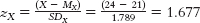 . Then calculate his predicted z score for number of hours studied: zŶ = (rXY)(zX) = (0.49)(1.677) = 0.82. Finally, translate the z score for hours studied into the raw score for hours studied: Ŷ = 0.82(5.582) + 14.2 = 18.777.
 - b. First, translate age raw score into an age z score:
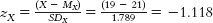 . Then calculate the predicted z score for hours studied: zŶ = (rXY)(zX) = (0.49)(−1.118) = −0.548. Finally, translate the z score for hours studied into the raw score for hours studied: Ŷ = −0.548(5.582) + 14.2 = 11.141.
 - c. Seung’s age is well above the mean age of the students sampled. The relation that exists for traditional-
aged students may not exist for students who are much older. Extrapolating beyond the range of the observed data may lead to erroneous conclusions. - d. From a mathematical perspective, the word regression refers to a tendency for extreme scores to drift toward the mean. In the calculation of regression, the predicted score is closer to its mean (i.e., less extreme) than the score used for prediction. For example, in part (a) the z score used for predicting was 1.677 and the predicted z score was 0.82, a less extreme score. Similarly, in part (b) the z score used for predicting was −1.118 and the predicted z score was −0.548—
again, a less extreme score. - e. First, we calculate what we would predict for Y when X equals 0; that number, −17.908, is the intercept.
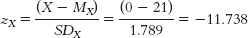

Note that the reason this prediction is negative (it doesn’t make sense to have a negative number of hours) is that the number for age, 0, is not a number that would actually be used in this situation—it’s another example of the dangers of extrapolation, but it still is necessary to determine the regression equation.
Then we calculate what we would predict for Y when X equals 1: the amount that that number, −16.378, differs from the prediction when X equals 0 is the slope.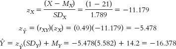
When X equals 0, −17.908 is the prediction for Y. When X equals 1, −16.378 is the prediction for Y. The latter number is 1.530 higher [−16.378 − (−17.908) = 1.530]—that is, more positive—than the former. Remember when you’re calculating the difference to consider whether the prediction for Y was more positive or more negative when X increased from 0 to 1.
Thus, the regression equation is: Ŷ = −17.91 + 1.53(X). - f. Substituting 17 for X in the regression equation for part (e) yields 8.1. Substituting 22 for X in the regression equation yields 15.75. We would predict that a 17-
year- old would study 8.1 hours and a 22- year- old would study 15.75 hours. - g. The accompanying graph depicts the regression line for predicting hours studied per week from a person’s age.
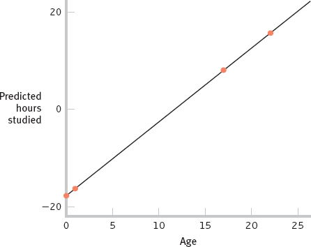
- h. It is misleading to include young ages such as 0 and 5 on the graph because people of that age would never be college students.
- i. The accompanying graph shows the scatterplot and regression line relating age and number of hours studied. Vertical lines from each observed data point are drawn to the regression line to represent the error prediction from the regression equation.
C-
62 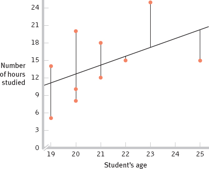
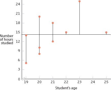
- j. The accompanying scatterplot relating age and number of hours studied includes a horizontal line at the mean number of hours studied. Vertical lines between the observed data points and the mean represent the amount of error in predicting from the mean.
- k. There appears to be less error in part (i), where the regression line is used to predict hours studied. This occurs because the regression line is the line that minimizes the distance between the observed scores and the line drawn through them. That is, the regression line is the one line that can be drawn through the data that produces the minimum error.
- l. To calculate the proportionate reduction in error the long way, we first calculate the predicted Y scores (3rd column) for each of the observed X scores in the data set and determine how much those predicted Y scores differ from the observed Y scores (4th column), and then we square them (5th column).We then calculate SSerror, which is the sum of the squared error when using the regression equation as the basis of prediction. This sum, calculated by adding the numbers in column 5, is 236.573. We then subtract the mean from each score (column 6), and square these differences (column 7).
AGE OBSERVED HOURS STUDIED PREDICTED HOURS STUDIED OBSERVED − PREDICTED SQUARE OF OBSERVED − PREDICTED OBSERVED − MEAN SQUARE OF OBSERVED − MEAN 19 5 11.16 −6.16 37.946 −9.2 84.64 20 20 12.69 7.31 53.436 5.8 33.64 20 8 12.69 −4.69 21.996 −6.2 38.44 21 12 14.22 −2.22 4.928 −2.2 4.84 21 18 14.22 3.78 14.288 3.8 14.44 23 25 17.28 7.72 59.598 10.8 116.64 22 15 15.75 −0.75 0.563 0.8 0.64 20 10 12.69 −2.69 7.236 −4.2 17.64 19 14 11.16 2.84 8.066 −0.2 0.04 25 15 20.34 −5.34 28.516 0.8 0.64 Next, we calculate SStotal, which is the sum of the squared error when using the mean as the basis of prediction. This sum is 311.6. Finally, we calculate the proportionate reduction in error asC-
63 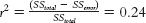 .
. - m. The r2 calculated in part (l) indicates that 24% of the variability in hours studied is accounted for by a student’s age. By using the regression equation, we have reduced the error of the prediction by 24% as compared with using the mean.
- n. To calculate the proportionate reduction in error the short way, we would square the correlation coefficient. The correlation between age and hours studied is 0.49. Squaring 0.49 yields 0.24. It makes sense that the correlation coefficient could be used to determine how useful the regression equation will be because the correlation coefficient is a measure of the strength of association between two variables. If two variables are strongly related, we are better able to use one of the variables to predict the values of the other.
- o. Here are the computations needed to compute β:
X (X − MX) (X − MX)2 Y (Y − MY) (Y − MY)2 19 −2 4 5 −9.2 84.64 20 −1 1 20 5.8 33.64 20 −1 1 8 −6.2 38.44 21 0 0 12 −2.2 4.84 21 0 0 18 3.8 14.44 23 2 4 25 10.8 116.64 22 1 1 15 0.8 0.64 20 −1 1 10 −4.2 17.64 19 −2 4 14 −0.2 0.04 25 4 16 15 0.8 0.64 Σ(X − MX)2 = 32 Σ(Y − MY)2 = 311.6 
- p. The standardized regression coefficient is equal to the correlation coefficient, 0.49, for simple linear regression.
- q. The hypothesis test for regression is the same as that for correlation. The critical values for r with 8 degrees of freedom at a p level of 0.05 are −0.632 and 0.632. With a correlation of 0.49, we fail to exceed the cutoff and therefore fail to reject the null hypothesis. The same is true then for the regression equation. We do not have a statistically significant regression and should be careful not to claim that the slope is different from 0.
- a. To predict the number of hours he studies per week, we use the formula zŶ = (rXY)(zX) to find the predicted z score for the number of hours he studies; then we can transform the predicted z score into his raw score. First, translate his predicted raw score for age into a z score for age: