Chapter 4
- 4.1 The mean is the arithmetic average of a group of scores; it is calculated by summing all the scores and dividing by the total number of scores. The median is the middle score of all the scores when a group of scores is arranged in ascending order. If there is no single middle score, the median is the mean of the two middle scores. The mode is the most common score of all the scores in a group of scores.
- 4.3 The mean takes into account the actual numeric value of each score. The mean is the mathematic center of the data. It is the center balance point in the data, such that the sum of the deviations (rather than the number of deviations) below the mean equals the sum of deviations above the mean.
- 4.5 The mean might not be useful in a bimodal or multimodal distribution because in a bimodal or multimodal distribution the mathematical center of the distribution is not the number that describes what is typical or most representative of that distribution.
- 4.7 The mean is affected by outliers because the numeric value of the outlier is used in the computation of the mean. The median typically is not affected by outliers because its computation is based on the data in the middle of the distribution, and outliers lie at the extremes of the distribution.
- 4.9 The standard deviation is the typical amount each score in a distribution varies from the mean of the distribution.
- 4.11 The standard deviation is a measure of variability in terms of the values of the measure used to assess the variable, whereas the variance is squared values. Squared values simply don’t make intuitive sense to us, so we take the square root of the variance and report this value, the standard deviation.
- 4.13 The range is the difference between the highest score and the lowest score in the data set. Thus, the range is completely driven by the most extreme scores in the data set and is susceptible to the effects of outliers. The interquartile range is based on the middle 50% of the data. Unlike the range, it is not affected by the effects of outliers.
- 4.15 The first quartile is the 25th percentile.
- 4.17
- a. The mean is calculated:
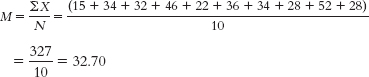
The median is found by arranging the scores in numeric order—15, 22, 28, 28, 32, 34, 34, 36, 46, 52— then dividing the number of scores, 10, by 2 and adding 1.2 to get 5.5. The mean of the 5th and 6th score in the ordered list of scores is the median— (32 + 34)/2 = 33— so 33 is the median.
The mode is the most common score. In these data, two scores appear twice, so we have two modes, 28 and 34. - b. Adding the value of 112 to the data changes the calculation of the mean in the following way:
(15 + 34 + 32 + 46 + 22 + 36 + 34 + 28 + 52 + 28 + 112)/11 = 439/11 = 39.91
The mean gets larger with this outlier.
There are now 11 data points, so the median is the 6th value in the ordered list, which is 34.
The modes are unchanged at 28 and 34.This outlier increases the mean by approximately 7 values; it increases the median by 1; and it does not affect the mode at all.C-
10 - c. The range is: Xhighest − Xlowest = 52 − 15 = 37
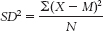
The variance is: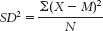
We start by calculating the mean, which is 32.70. We then calculate the deviation of each score from the mean and the square of that deviation.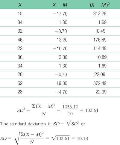
- a. The mean is calculated:
- 4.19
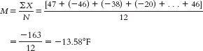
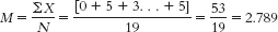
- a. The mean is calculated as:
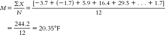
The median is found by arranging the temperatures in numeric order:
−3.7, −1.7, 1.7, 5.9, 13.6, 16.4, 24, 29.5, 34.6, 38.5, 42.1, 43.3
There are 12 data points, so the mean of the 6th and 7th data points gives us the median: (16.4 + 24)/2 + 20.20°F. - b. The mean is calculated as:
The median is found by arranging the temperatures in numeric order:
−47, −46, −46, −38, −20, −20, −5, −2, 8, 9, 20, 24
There are 12 data points, so the mean of the 6th and 7th data points gives us the median: [−20 + −5]/2 = −25/2 = −12.50°F.
There are two modes: both −46 and −20 were recorded twice. - c. The mean is calculated as:
The median is found by arranging the wind gusts in numeric order:
136, 142, 154, 161, 163, 164, 166, 173, 174, 178, 180, 231
There are 12 data points, so the mean of the 6th and 7th data points gives us the median: (164 + 166)/2 = 165 mph.
There is no mode among these wind gusts. - d. For the wind gust data, we could create 10-
mph intervals and calculate the mode as the interval that occurs most often. There are four recorded gusts in the 160– 169 mph interval, three in the 170– 179 interval, and only one in the other intervals. So, the 160– 169 mph interval could be presented as the mode. - e. The range is: Xhighest − Xlowest = 43.3 − (−3.7) = 47°F
The variance is:
We start by calculating the mean, which is 20.35°F. We then calculate the deviation of each score from the mean and the square of that deviation.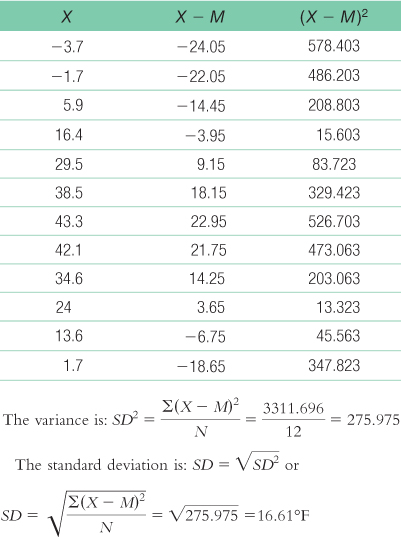
- f. The range is Xhighest − Xlowest = 24 − (−47) = 71°F
The variance is:
We already calculated the mean, −13.583°F. We now calculate the deviation of each score from the mean and the square of that deviation.C-
11 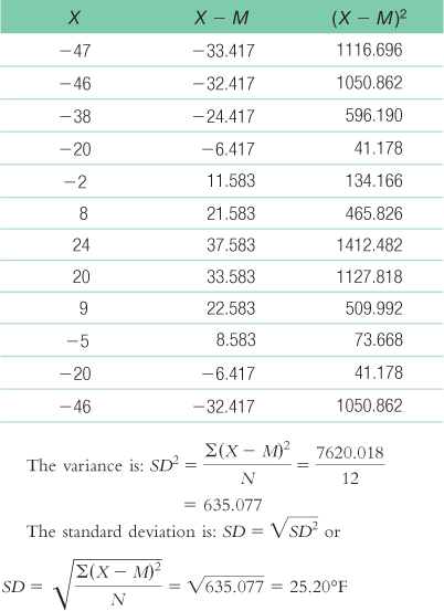
- g. For the peak wind gust data, the range is Xhighest − Xlowest = 231 − 136 = 95 mph
The variance is: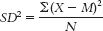
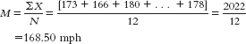
We start by calculating the mean, which is 168.50 mph. We then calculate the deviation of each score from the mean and the square of that deviation.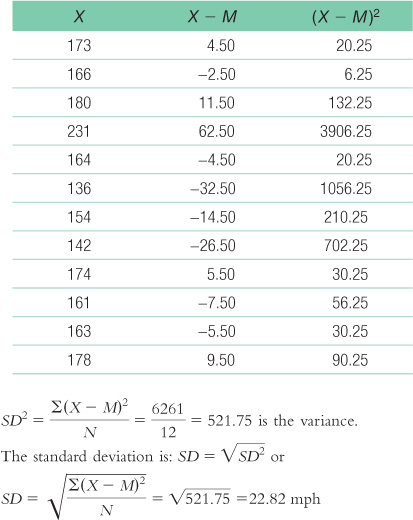
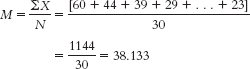
- a. The mean is calculated as:
- 4.21 Calculating the interquartile range requires that we order the observations from lowest to highest, find the first and third quartiles, and subtract the first from the third. Here are the data sorted from lowest to highest:
1 1 1 2 2 2 2 3 3 3 3 3 3 4 4 5 6 7 7 8 12
Q1 is the median of the first half of the observations, which is 2. Q3 is the median of the second half of the observations, which is 5.50. The IQR = Q3 − Q1, or IQR = 5.50 − 2 = 3.50. - 4.23 The interquartile range of 18.50 is so much smaller than the range of 95 because there is an outlier of 231 mph in the wind gust data. This outlier affects the range but not the interquartile range.
- 4.25 The mean for salary is often greater than the median for salary because the high salaries of top management inflate the mean but not the median. If we are trying to attract people to our company, we may want to present the typical salary as whichever value is higher—
in most cases, the mean. However, if we are going to offer someone a low salary, presenting the median might make them feel better about that amount! - 4.27 There are few participants in this study (only seven) so a single extreme score would influence the mean more than it would influence the median. The median is a more trustworthy indicator than the mean when there is only a handful of scores.
- 4.29 In April 1934, a wind gust of 231 mph was recorded. This data point is rather far from the next closest record of 180 mph. If this extreme score were excluded from analyses of central tendency, the mean would be lower, the median would change only slightly, and the mode would be unaffected.
- 4.31 There are many possible answers to this question. All answers will include a distribution that is skewed, perhaps one that has outliers. A skewed distribution would affect the mean but not the median. One example would be the variable of number of foreign countries visited; the few jet-
setters who have been to many countries would pull the mean higher. The median is more representative of the typical score. - 4.33
- a. These ads are likely presenting outlier data.
- b. To capture the experience of the typical individual who uses the product, the ad could include the mean result and the standard deviation. If the distribution of outcomes is skewed, it would be best to present the median result.
- 4.35
- a.
- b. The formula for variance is
 We start by creating three columns: one for the scores, one for the deviations of the scores from the mean, and one for the squares of the deviations.
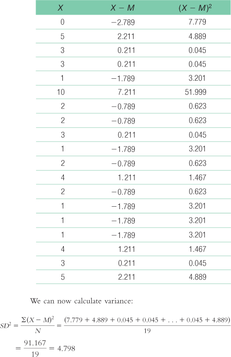
C-
12 - c. Standard deviation is calculated just like we calculated variance, but we then take the square root:
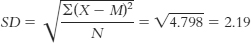
- d. The typical score is around 2.79, and the typical deviation from 2.79 is around 2.19.
- a.
- 4.37 There are many possible answers to these questions. The following are only examples.
- a. 70, 70. There is no skew; the mean is not pulled away from the median.
- b. 80, 70. There is positive skew; the mean is pulled up, but the median is unaffected.
- c. 60, 70. There is negative skew; the mean is pulled down, but the median is unaffected.
- 4.39
- a. Because the policy for which violations were issued changed during this time frame, we cannot make accurate comparisons before and after Hurricane Sandy. The conditions for issuing violations were not constant; thus, the policy change would be a likely explanation for a change in the data.
- b. The removal of violations in Zone A, which appears to have been most affected by infestations after the hurricane, would result in eliminating an otherwise extreme number, or outlier, of issued violations. This would lead to inaccurate data as it does not accurately portray the number of rat violations, only the number of rat violations issued under the current policy.
- 4.41 It would probably be appropriate to use the mean because the data are scale; we would assume we have a large number of data points available to us; and the mean is the most commonly used measure of central tendency. Because of the large amount of data available, the effect of outliers is minimized. All of these factors would support the use of the mean for presenting information about the heights or weights of large numbers of people.
- 4.43 We cannot directly compare the mean ages reported by Canada with the median ages reported by the United States because it is likely that there were some older outliers in both Canada and the United States, and these outliers would affect the means reported by Canada much more than they would affect the medians reported by the United States.
- 4.45
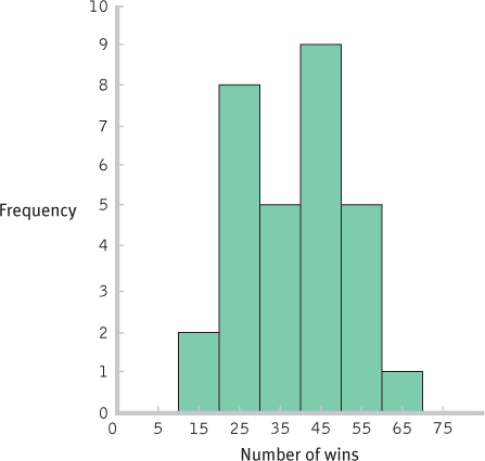
- a.
INTERVAL FREQUENCY 60– 69 1 50– 59 5 40– 49 9 30– 39 5 20– 29 8 10– 19 2 - b.
- c.
With 30 scores, the median would be between the 15th and 16th scores: (30/2) + 0.5 + 15.5. The 15th and 16th scores are 39 and 40, respectively, so the median is 39.50. The mode is 29; there are three scores of 29. - d. Software reports that the range is 42 and the standard deviation is 11.59.
- e. The summary will differ for each student but should include the following information: The data appear to be roughly symmetric and unimodal, maybe a bit negatively skewed. There are no glaring outliers.
- f. Answers will vary. One example is whether number of wins is related to the average age of a team’s players.
- a.
C-