9.1 The t statistic indicates the distance of a sample mean from a population mean in terms of the estimated standard error.
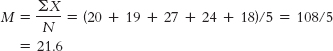
9.2 First we need to calculate the mean: We then calculate the deviation of each score from the mean and the square of that deviation.
X
X − M
(X − M)2
6
0.833
0.694
3
−2.167
4.696
7
1.833
3.360
6
0.833
0.694
4
−1.167
1.362
5
−0.167
0.028
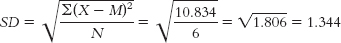
The standard deviation is:
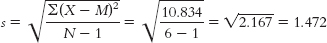
When estimating the population variability, we calculate s:
9.3
9.4
a. We would use a distribution of means, specifically a t distribution. It is a distribution of means because we have a sample consisting of more than one individual. It is a t distribution because we are comparing one sample to a population, but we know only the population mean, not its standard deviation.
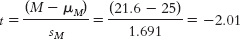
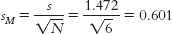
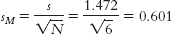
b. The appropriate mean: μM = μ = 25. The calculations for the appropriate standard deviation (in this case, standard error, sM):
9.5Degrees of freedom is the number of scores that are free to vary, or take on any value, when a population parameter is estimated from a sample.
9.6 A single-sample t test is more useful than a z test because it requires only that we know the population mean (not the population standard deviation).
9.7
a.df = N − 1 = 35 − 1 = 34
b.df = N − 1 = 14 − 1 = 13
9.8
a. ±2.201
b. Either −2.584 or +2.584, depending on the tail of interest
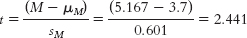
9.9Step 1: Population 1 is the sample of six students. Population 2 is all university students. The distribution will be a distribution of means, and we will use a single-sample t test. We meet the assumption that the dependent variable is scale. We do not know if the sample was randomly selected, and we do not know if the population variable is normally distributed. Some caution should be exercised when drawing conclusions from these data. Step 2: The null hypothesis is H0: μ1 = μ2; that is, students we’re working with miss the same number of classes, on average, as the population. The research hypothesis is H1: μ1 ≠ μ2; that is, students we’re working with miss a different number of classes, on average, than the population. Step 3: μM = μ = 3.7 Step 4: df = N − 1 = 6 − 1 = 5 For a two-tailed test with a p level of 0.05 and 5 degrees of freedom, the cutoffs are ±2.571. Step 5: Step 6: Because the calculated t value falls short of the critical values, we fail to reject the null hypothesis.

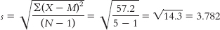
 When estimating the population variability, we calculate s:
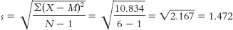
 Numerator: Σ(X − M)2 = (2.56 + 6.76 + 29.16 + 5.76 + 12.96) = 57.2