Chapter 11 How it Works
11.1 Independent-Samples t Test
Who do you think have a better sense of humor—
However, the researchers were aware of other possible explanations for these findings. For example, they considered whether one gender is more likely to find humorous stimuli funny to begin with. In this study, men and women indicated the percentage of 30 cartoons that they perceived to be either “funny” or “unfunny.” Below are fictional data for nine people (four women and five men); these fictional data have approximately the same means as in the original study.
- Percentage of cartoons labeled as “funny”
- Women: 84, 97, 58, 90
- Men: 88, 90, 52, 97, 86
How can we conduct all six steps of hypothesis testing for an independent-
- Population 1: Women exposed to humorous cartoons. Population 2: Men exposed to humorous cartoons.
The comparison distribution will be a distribution of differences between means based on the null hypothesis. The hypothesis test will be an independent-samples t test because we have two samples composed of different groups of participants. This study meets one of the three assumptions. (1) The dependent variable is a percentage of cartoons categorized as “funny,” which is a scale variable. (2) We do not know whether the population is normally distributed, and there are not at least 30 participants. Moreover, the data suggest some negative skew; although this test is robust with respect to this assumption, we must be cautious. (3) The men and women in this study were not randomly selected from among all men and women, so we must be cautious with respect to generalizing these findings. - Null hypothesis: On average, women categorize the same percentage of cartoons as “funny” as men—
H0: μ1 = μ2. Research hypothesis: On average, women categorize a different percentage of cartoons as “funny” as compared with men— H1: μ1 ≠ μ2. - (μ1 − μ2) = 0; sdifference = 11.641
Calculations:- MX = 82.25
X X − M (X −M)2 84 1.75 3.063 97 14.75 217.563 58 −24.25 588.063 90 7.75 60.063 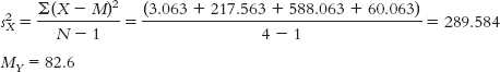
280
Y Y −M (Y −M)2 88 5.4 29.16 90 7.4 54.76 52 −30.6 936.36 97 14.4 207.36 86 3.4 11.56 
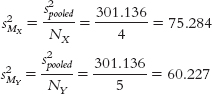
- dfX = N − 1 = 4 − 1 = 3
dfY = N − 1 = 5 − 1 = 4
dftotal = dfX + dfY = 3 + 4 = 7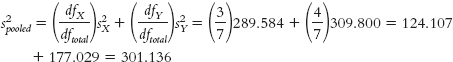


- MX = 82.25
- The critical values, based on a two-
tailed test, a p level of 0.05, and a dftotal of 7, are −2.365 and 2.365 (as seen in the curve in Figure 11-2 on page 269). 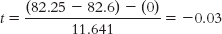
- Fail to reject the null hypothesis. We conclude that there is no evidence from this study to support the research hypothesis that either men or women are more likely than the opposite gender, on average, to find cartoons funny.
11.2 Reporting The Statistics in a Journal
How would we report the results of the hypothesis test described in How It Works 11.1? The statistics would appear in a journal article as: t(7) = −0.03, p > 0.05. In addition to the results of hypothesis testing, we would also include the means and standard deviations for the two samples. We calculated the means in step 3 of hypothesis testing, and we also calculated the variances. We can calculate the standard deviations by taking the square roots of the variances. The descriptive statistics can be reported in parentheses as:
(Women: M = 82.25, SD = 17.02; Men: M = 82.60, SD = 17.60)
11.3 Confidence Intervals for an Independent-Samples t Test
How would we calculate a 95% confidence interval for the independent-
Previously, we calculated the difference between the means of these samples to be 82.25 − 82.6 = −0.35; the standard error for the differences between means, sdifference, to be 11.641; and the degrees of freedom to be 7. (Note that the order of subtraction in calculating the difference between means is irrelevant; we could just as easily have subtracted 82.25 from 82.6 and gotten a positive result, 0.35.)
- We draw a normal curve with the sample difference between means in the center.
- We indicate the bounds of the 95% confidence interval on either end and write the percentages under each segment of the curve—
2.5% in each tail. - We look up the t statistics for the lower and upper ends of the confidence interval in the t table, based on a two-
tailed test, a p level of 0.05 (which corresponds to a 95% confidence interval), and the degrees of freedom— 7— that we calculated earlier. Because the normal curve is symmetric, the bounds of the confidence interval fall at t statistics of −2.365 and 2.365. We add those t statistics to the normal curve. - We convert the t statistics to raw differences between means for the lower and upper ends of the confidence interval.
(MX −MY)lower = −t(sdifference) + (MX −MY)sample = −2.365(11.641) + (−0.35) = −27.88
(MX − MY)upper = t(sdifference) + (MX − MY)sample = 2.365(11.641) + (−0.35) = 27.18
The confidence interval is [−27.88, 27.18]. - We check the answer; each end of the confidence interval should be exactly the same distance from the sample mean.
−27.88 − (−0.35) = −27.53
27.18 − (−0.35) = 27.53
The interval checks out, and we know that the margin of error is 27.53.
11.4 Effect Size for an Independent-Samples t Test
How can we calculate an effect size for the independent-
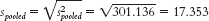
For Cohen’s d, we simply replace the denominator of the formula for the test statistic with the standard deviation, spooled, instead of the standard error, sdifference.

According to Cohen’s conventions, this is not even near the level of a small effect.