12.1 Using the F Distributions with Three or More Samples

The self-esteem experiment revealed the possible dangers of building self-esteem because the researchers compared two groups with two different ways of motivating students to a third group, a control group. A three-group comparison is slightly more complicated than a two-group comparison, so it requires comparison distributions that can accommodate that complexity: the F distributions.

Type I Errors When Making Three or More Comparisons

When comparing three or more groups, it is tempting to conduct an easy-to-understand t test on each of the possible comparisons. Unfortunately, there’s a big downside: You may not be able to believe your own results. Why? Conducting numerous t tests greatly increases the probability of a Type I error (a false positive: rejecting the null hypothesis when the null hypothesis is true). The three possible comparisons in the self-esteem experiment demonstrate why conducting many t tests inflates the possibility of making a Type I error:

• Group 1 with group 2
• Group 1 with group 3
• Group 2 with group 3

That’s 3 comparisons, and if there were four groups, there would be 6 comparisons. With five groups, there would be 10 comparisons, and so on. With only 1 comparison, there is a 0.05 chance of having a Type I error in any given analysis if the null hypothesis is true, and a 0.95 chance of not having a Type I error when the null hypothesis is true. Those are pretty good odds, and we would tend to believe the conclusions in that study. However, Table 12-1 shows what happens when we conduct more studies on the same sample. The chances of not having a Type I error on the first analysis and not having a Type I error on the second analysis are (0.95)(0.95) = (0.95)² = 0.903, or about 90%. This means that the chance of having a Type I error is almost 10%. With three analyses, the chance of not having a Type I error is (0.95) (0.95)(0.95) = (0.95)³ = 0.857, or about 86%. This means that there is about a 14% chance of having at least one Type I error. And so on, as we see in Table 12-1. ANOVA is a more powerful approach because it lets us test differences among three or more groups in just one test.

The F Statistic as an Expansion of the z and t Statistics

z, t, and F Distributions The z, t, and F distributions are three increasingly complex variations on one great idea: the normal curve.

© Simon Belcher/Alamy
Simple Stock Shots/IPNStock
© Nick Emm/Alamy

We use F distributions because they allow us to conduct a single hypothesis test with multiple groups. F distributions are more conservative versions of the z distribution and the t distributions. Just as the z distribution is still part of the t distributions, the t distributions are also part of the F distributions—and they all rely on the characteristics of the normal bell-shaped curve. The distributions are like progressively more complex versions of the Swiss Army knife: The z distribution has just one blade; the t distributions add a second blade; and the versatile F distributions can do everything the z and the t can do—as well as many more complex statistical tasks.

The hypothesis tests that we have learned so far—the z test and the three types of t tests—are calculated in similar ways. The numerator describes how far apart comparison groups are from each other (between-groups variability); the denominator describes other sources of variability, such as individual differences and chance (within-groups variability). For example, the average height of men is greater than the average height of women: between-groups variability. Yet not all men are the same height and not all women are the same height: within-groups variability. However, many women are taller than many men, so there is considerable overlap between the two distributions. The F statistic calculates between-group and within-group variance to conduct the hypothesis test called analysis of variance (ANOVA; pronounced “ah-no-vah”), a hypothesis test typically used with one or more nominal (and sometimes ordinal) independent variables (with at least three groups overall) and a scale dependent variable.

The F Distributions for Analyzing Variability to Compare Means

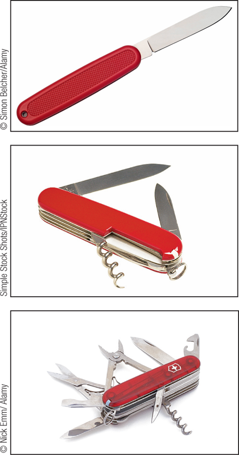
Comparing the height between men and women demonstrates that the F statistic is a ratio of two measures of variance: (1) between-groups variance, which indicates differences among sample means, and (2) within-groups variance, the average of the sample variances.

Let’s begin with the numerator, called between-groups variance because it is an estimate of the population variance, based on the differences among the means. A big number in the numerator indicates a great deal of distance (or spread) between the means, suggesting that they come from different populations. A small number in the numerator indicates very little distance (or spread) between the means, suggesting that they come from the same population. With more than two means, we can’t use simple subtraction to find a number that indicates how spread apart they are, so we calculate the variance among the sample means. For example, if we wanted to compare how fast people talk in Vancouver, Memphis, Chicago, and Toronto, then the number representing between-groups variance (in this case, the between-cities variance) is an estimate of the variability among the average number of words per minute spoken by the people representing each of those four cities.

The denominator of the F statistic is called the within-groups variance, an estimate of the population variance, based on the differences within each of the three (or more) sample distributions. For example, not everyone living in Vancouver, Memphis, Chicago, or Toronto speaks at the same pace. There are within-city differences in talking speeds, so within-groups variance refers to the average of the four variances.

To calculate the F statistic, we simply divide the between-groups variance by the within-groups variance. If the F statistic is a large number (when the between-groups variance is much larger than the within-groups variance), then we can infer that the sample means are different from one another. But we cannot make that inference when the F statistic is close to the number 1 (the between-groups variance is about the same as the within-groups variance).

To summarize, we can think of within-groups variance as reflecting the difference between means that we’d expect just by chance. There is variability within any population, so we would expect some difference among means just by chance. Between-groups variance reflects the difference between means that we found in the data. If this difference is much larger than the within-groups variance—what we’d expect by chance—then we can reject the null hypothesis and conclude that there is some difference between means.

The F Table

The F table is an expansion of the t table. Just as there are many t distributions represented in the t table—one for each possible sample size—there are many F distributions. Both tables include a wide range of sample sizes (represented by degrees of freedom) but the F table adds a third factor: the number of samples. (The t statistic is limited to two samples.) There is an F distribution for every possible combination of sample size (represented by one type of degrees of freedom) and number of samples (represented by another type of degrees of freedom).

The F table for two samples can even be used as a t test; the numbers are the same except that the F is based on variance and the t on the square root of the variance, the standard deviation. For example, if we look in the F table under two samples for a sample size of infinity for the equivalent of the 95th percentile, we see 2.71. If we take the square root of this, we get 1.646. We can find 1.645 on the z table for the 95th percentile and on the t table for the 95th percentile with a sample size of infinity. (The slight differences are due only to rounding decisions.) The connections between the z, t, and F distributions are summarized in Table 12-2.

The Language and Assumptions for ANOVA

Here is a simple guide to the language that statisticians use to describe different kinds of ANOVAs (Landrum, 2005). The word ANOVA is almost always preceded by two adjectives that indicate: (1) the number of independent variables; and (2) the research design (between-groups or within-groups).

Study 1. What would you call an ANOVA with year in school as the only independent variable and Consideration of Future Consequences (CFC) scores as the dependent variable? Answer: A one-way between-groups ANOVA. A one-way ANOVA is a hypothesis test that includes both one nominal independent variable with more than two levels and a scale-dependent variable. A between-groups ANOVA is a hypothesis test in which there are more than two samples, and each sample is composed of different participants.

Study 2. What if you wanted to test the same group of students every year? Answer: You would use a one-way within-groups ANOVA. A within-groups ANOVA is a hypothesis test in which there are more than two samples, and each sample is composed of the same participants. (This test is also called a repeated-measures ANOVA.)

Study 3. And what if you wanted to add gender to the first study, something we explore in the next chapter? Now you have two independent variables: year in school and gender. Answer: You would use a two-way between-groups ANOVA.

All ANOVAs, regardless of type, share the same three assumptions that represent the optimal conditions for valid data analysis.

Assumption 1. Random selection is necessary if we want to generalize beyond a sample. Because of the difficulty of random sampling, researchers often substitute convenience sampling and then replicate their experiment with a new sample.

Assumption 2. A normally distributed population allows us to examine the distributions of the samples to get a sense of what the underlying population distribution might look like. This assumption becomes less important as the sample size increases.

Assumption 3. Homoscedasticity (also called homogeneity of variance) assumes that the samples all come from populations with the same variances. (Heteroscedasticity means that the populations do not all have the same variance.) Homoscedastic populations are those that have the same variance. Heteroscedastic populations are those that have different variances. (Note that homoscedasticity is also often called homogeneity of variance.)

What if your study doesn’t match these ideal conditions? You may have to throw away your data—but that is usually not necessary. You also can (a) report and justify your decision to violate those assumptions; or (b) conduct a more conservative nonparametric test (see Chapter 18).