13.1 One-Way Within-Groups ANOVA
There is not much difference between chapters 12 and 13. Chapter 12 taught you how to conduct the multiple-
EXAMPLE 13.1
Have you ever participated in a taste test? If you have, then you were probably a participant in a within-
329

Fallows wanted to know whether his recruits could distinguish among widely available American beers that were categorized into three groups based on price—
| Participant | Cheap Beer | Mid- |
High- |
|---|---|---|---|
| 1 | 40 | 30 | 53 |
| 2 | 42 | 45 | 65 |
| 3 | 30 | 38 | 64 |
| 4 | 37 | 32 | 43 |
| 5 | 23 | 28 | 38 |
MASTERING THE CONCEPT
13.1: We use a one-
The Benefits of Within-Groups ANOVA
Fallows only reported his overall findings. If he had conducted hypothesis testing, then he would have used a one-
MASTERING THE CONCEPT
13.2: The calculations for a one-
The beauty of the within-
330
The Six Steps of Hypothesis Testing
EXAMPLE 13.2
We’ll use the data from the beer taste test to walk through the same six steps of hypothesis testing that you have used for every other statistical test.
STEP 1: Identify the populations, distribution, and assumptions.
The one-
Summary: Population 1: People who drink cheap beer. Population 2: People who drink mid-
The comparison distribution and hypothesis test: The comparison distribution is an F distribution. The hypothesis test is a one-
Assumptions: (1) The participants were not selected randomly, so we must generalize with caution. (2) We do not know if the underlying population distributions are normal, but the sample data do not indicate severe skew. (3) After we calculate the test statistic, we will test the homoscedasticity assumption by checking to see whether the largest variance is more than twice the smallest. (4) The experimenter did not counterbalance, so there may be order effects.
STEP 2: State the null and research hypotheses.
This step is identical to that for a one-
Summary: Null hypothesis: People who drink cheap, mid-
STEP 3: Determine the characteristics of the comparison distribution.
We state that the comparison distribution is an F distribution and determine the degrees of freedom. Instead of three, we now calculate four kinds of degrees of freedom—
We calculate the between-
dfbetween = Ngroups − 1 = 3 − 1 = 2
331
We next calculate the degrees of freedom that pairs with SSsubjects. Called dfsubjects, it is calculated by subtracting 1 from the actual number of subjects, not from the number of data points. We use a lowercase n to indicate that this is the number of participants in a single sample (even though they’re all in every sample). The formula is:
MASTERING THE FORMULA
13-
dfsubjects = n − 1 = 5 − 1 = 4
Once we know the between-
MASTERING THE FORMULA
![]() 13-
13-
dfwithin = (dfbetween)(dfsubjects) = (2)(4) = 8
Note that the within-
Finally, we calculate total degrees of freedom using either method we learned earlier. We can sum the other degrees of freedom:
dftotal = dfbetween + dfsubjects + dfwithin = 2 + 4 + 8 = 14
Alternatively, we can use the second formula we learned before, treating the total number of participants as every data point, rather than every person. We know, of course, that there are just five participants and that they participate in all three levels of the independent variable, but for this step, we count the 15 total data points:
MASTERING THE FORMULA
13-
dftotal = Ntotal − 1 = 15 − 1 = 14
We have calculated the 4 degrees of freedom that we will include in the source table. However, we only report the between-
Summary: We use the F distribution with 2 and 8 degrees of freedom.
STEP 4: Determine the critical values, or cutoffs.
The fourth step is identical to that for a one-
Summary: The critical value for the F statistic for a p level of 0.05 and 2 and 8 degrees of freedom is 4.46.
STEP 5: Calculate the test statistic.
As before, we calculate the test statistic in the fifth step. To start, we calculate four sums of squares—
332
As we did with the one-
SStotal = Σ(X − GM)2 = 2117.732
| Type of Beer | Rating (X) | X − GM | (X − GM)2 |
|---|---|---|---|
| Cheap | 40 | −0.533 | 0.284 |
| Cheap | 42 | 1.467 | 2.152 |
| Cheap | 30 | −10.533 | 110.944 |
| Cheap | 37 | −3.533 | 12.482 |
| Cheap | 23 | −17.533 | 307.406 |
| Mid- |
30 | −10.533 | 110.944 |
| Mid- |
45 | 4.467 | 19.954 |
| Mid- |
38 | −2.533 | 6.416 |
| Mid- |
32 | −8.533 | 72.812 |
| Mid- |
28 | −12.533 | 157.076 |
| High- |
53 | 12.467 | 155.426 |
| High- |
65 | 24.467 | 598.634 |
| High- |
64 | 23.467 | 550.700 |
| High- |
43 | 2.467 | 6.086 |
| High- |
38 | −2.533 | 6.416 |
| GM = 40.533 Σ(X − GM)2 = 2117.732 | |||
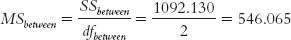
Next, we calculate the between-
SSbetween = Σ(M − GM)2 = 1092.130
| Type of Beer | Rating (X) | Group mean (M) | M − GM | (M − GM)2 |
|---|---|---|---|---|
| Cheap | 40 | 34.4 | −6.133 | 37.614 |
| Cheap | 42 | 34.4 | −6.133 | 37.614 |
| Cheap | 30 | 34.4 | −6.133 | 37.614 |
| Cheap | 37 | 34.4 | −6.133 | 37.614 |
| Cheap | 23 | 34.4 | −6.133 | 37.614 |
| Mid- |
30 | 34.6 | −5.933 | 35.200 |
| Mid- |
45 | 34.6 | −5.933 | 35.200 |
| Mid- |
38 | 34.6 | −5.933 | 35.200 |
| Mid- |
32 | 34.6 | −5.933 | 35.200 |
| Mid- |
28 | 34.6 | −5.933 | 35.200 |
| High- |
53 | 52.6 | 12.067 | 145.612 |
| High- |
65 | 52.6 | 12.067 | 145.612 |
| High- |
64 | 52.6 | 12.067 | 145.612 |
| High- |
43 | 52.6 | 12.067 | 145.612 |
| High- |
38 | 52.6 | 12.067 | 145.612 |
| GM = 40.533 Σ(M − GM)2 = 1092.130 | ||||
333
MASTERING THE FORMULA
![]() 13-
13-
So far, the calculations of the sums of squares for a one-
So the formula for the subjects sum of squares is:
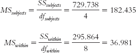
SSsubjects = Σ(Mparticipant − GM)2 = 729.738
| Participant | Type of Beer | Rating (X) | Participant Mean (Mparticipant) | Mparticipant − GM | (Mparticipant − GM)2 |
|---|---|---|---|---|---|
| 1 | Cheap | 40 | 41 | 0.467 | 0.218 |
| 2 | Cheap | 42 | 50.667 | 10.134 | 102.698 |
| 3 | Cheap | 30 | 44 | 3.467 | 12.02 |
| 4 | Cheap | 37 | 37.333 | −3.2 | 10.24 |
| 5 | Cheap | 23 | 29.667 | −10.866 | 118.07 |
| 1 | Mid- |
30 | 41 | 0.467 | 0.218 |
| 2 | Mid- |
45 | 50.667 | 10.134 | 102.698 |
| 3 | Mid- |
38 | 44 | 3.467 | 12.02 |
| 4 | Mid- |
32 | 37.333 | −3.2 | 10.24 |
| 5 | Mid- |
28 | 29.667 | −10.866 | 118.07 |
| 1 | High- |
53 | 41 | 0.467 | 0.218 |
| 2 | High- |
65 | 50.667 | 10.134 | 102.698 |
| 3 | High- |
64 | 44 | 3.467 | 12.02 |
| 4 | High- |
43 | 37.333 | −3.2 | 10.24 |
| 5 | High- |
38 | 29.667 | −10.866 | 118.07 |
| GM = 40.533 Σ(Mparticipant − GM)2 = 729.738 | |||||
We only have one sum of squares left to go. To calculate the within-
MASTERING THE FORMULA
13-
SSwithin = SStotal − SSbetween − SSsubjects
= 2117.732 − 1092.130 − 729.738 = 295.864
We now have enough information to fill in the first three columns of the source table—
MASTERING THE FORMULA
13-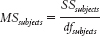 .
.
334
We then calculate two F statistics—
MASTERING THE FORMULA
![]() 13-
13- . We divide the subjects mean square by the within-
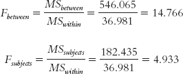
The completed source table is shown here:
| Source | SS | df | MS | F |
|---|---|---|---|---|
| Between- |
1092.130 | 2 | 546.065 | 14.766 |
| Subjects | 729.738 | 4 | 182.435 | 4.933 |
| Within- |
295.864 | 8 | 36.981 | |
| Total | 2117.732 | 14 |
Here is a recap of the formulas used to calculate a one-
| Source | SS | df | MS | F |
|---|---|---|---|---|
| Between- |
Σ(M − GM)2 | Ngroups − 1 |

|

|
| Subjects | Σ(Mparticipant − GM)2 | dfsubjects = n − 1 |

|

|
| Within- |
SStotal − SSbetween − SSsubjects | (dfbetween) (dfsubjects) |

|
|
| Total | Σ(X − GM)2 | Ntotal − 1 |
We calculated two F statistics, but we’re really only interested in the between-
Summary: The F statistic associated with the between-
STEP 6: Make a decision.
This step is identical to that for the one-
Summary: The F statistic, 14.77, is beyond the critical value, 4.46. We reject the null hypothesis. It appears that mean ratings of beers differ based on the type of beer in terms of price category, although we cannot yet know exactly which means differ. We report the statistics in a journal article as F(2,8) = 14.77, p < 0.05. (Note: If we used software, we would report the exact p value.)
335
CHECK YOUR LEARNING
Reviewing the Concepts
- We use one-
way within- groups ANOVA when we have a nominal or ordinal independent variable with at least three levels, a scale dependent variable, and participants who experience all levels of the independent variable. - Because all participants experience all levels of the independent variable, we reduce the within-
groups variability by reducing individual differences; each person serves as a control for him- or herself. A possible concern with this design is order effects. - One-
way within- groups ANOVA uses the same six steps of hypothesis testing that are used for one- way between- groups ANOVA— with one major exception. We calculate statistics for four sources rather than three. The fourth source, which is in addition to between- groups, within- groups, and total, is typically called “subjects.”
Clarifying the Concepts
- 13-
1 Why is the within-groups variability, or sum of squares, smaller for the within- groups ANOVA compared to the between- groups ANOVA?
Calculating the Statistics
- 13-
2 Calculate the four degrees of freedom for the following groups, assuming a within-groups design: Participant 1 Participant 2 Participant 3 Group 1 7 9 8 Group 2 5 8 9 Group 3 6 4 6 - dfbetween = Ngroups − 1
- dfsubjects = n − 1
- dfwithin = (dfbetween)(dfsubjects)
- dftotal = dfbetween + dfsubjects + dfwithin; or dftotal = Ntotal − 1
- 13-
3 Calculate the four sums of squares for the data in Check Your Learning 13-2: - SStotal = Σ(X − GM)2
- SSbetween = Σ(M − GM)2
- SSsubjects = Σ(Mparticipant − GM)2
- SSwithin = SStotal − SSbetween − SSsubjects
- 13-
4 Using all of your calculations in Check Your Learning 13-2 and 13- 3, perform the simple division to complete an ANOVA source table for these data.
Applying the Concepts
- 13-
5 Let’s create a context for the data presented in Check Your Learning 13-2. Suppose a car dealer wants to sell a car by having people test drive it and two other cars in the same class (e.g., midsize sedans). The data from these three groups might represent the ratings, ranging from 1 (low quality) to 10 (high quality), that drivers gave the driving experience after test- driving the cars. Using the F values you calculated above, complete the following: - Write hypotheses, in words, for this study.
- How might you conduct this research such that you would satisfy the fourth assumption of the within-
groups ANOVA? - Determine the critical value for F and make a decision about the outcome of this research.
Solutions to these Check Your Learning questions can be found in Appendix D.
336