Chapter 15 Exercises
Clarifying the Concepts
Question 15.1
What is a correlation coefficient?
Question 15.2
What is a linear relation?
Question 15.3
Describe a perfect correlation, including its possible coefficients.
Question 15.4
What is the difference between a positive correlation and a negative correlation?
Question 15.5
What magnitude of a correlation coefficient is large enough to be considered important, or worth talking about?
Question 15.6
When we have a straight-
Question 15.7
Explain how the correlation coefficient can be used as a descriptive or an inferential statistic.
Question 15.8
How are deviation scores used in assessing the relation between variables?
Question 15.9
Explain how the sum of the product of deviations determines the sign of the correlation.
Question 15.10
What are the null and research hypotheses for correlations?
Question 15.11
What are the three basic steps to calculate the Pearson correlation coefficient?
Question 15.12
Describe the third assumption of hypothesis testing with correlation.
Question 15.13
What is the difference between test–
Question 15.14
Why is a correlation coefficient never greater than 1 (or less than −1)?
Question 15.15
In your own words, briefly explain the difference between a Pearson correlation coefficient and a partial correlation coefficient.
Question 15.16
How does partial correlation begin to address the third variable problem?
412
Calculating the Statistics
Question 15.17
Determine whether the data in each of the graphs provided would result in a negative or positive correlation coefficient.
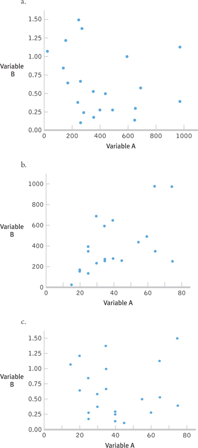
Question 15.18
Decide which of the three correlation coefficient values below goes with each of the scatterplots presented in Exercise 15.17.
0.545
0.018
−0.20
Question 15.19
Use Cohen’s guidelines to describe the strength of the following correlation coefficients:
−0.28
0.79
1.0
−0.015
Question 15.20
For each of the pairs of correlation coefficients provided, determine which one indicates a stronger relation between variables:
−0.28 and −0.31
0.79 and 0.61
1.0 and −1.0
−0.15 and 0.13
Question 15.21
Using the following data:
| X | Y |
|---|---|
| 0.13 | 645 |
| 0.27 | 486 |
| 0.49 | 435 |
| 0.57 | 689 |
| 0.84 | 137 |
| 0.64 | 167 |
Create a scatterplot.
Calculate deviation scores and products of the deviations for each individual, and then sum all products. This is the numerator of the correlation coefficient equation.
Calculate the sum of squares for each variable. Then compute the square root of the product of the sums of squares. This is the denominator of the correlation coefficient equation.
Divide the numerator by the denominator to compute the coefficient, r.
Calculate degrees of freedom.
Determine the critical values, or cutoffs, assuming a two-
tailed test with a p level of 0.05.
413
Question 15.22
Using the following data:
| X | Y |
|---|---|
| 394 | 25 |
| 972 | 75 |
| 349 | 25 |
| 349 | 65 |
| 593 | 35 |
| 276 | 40 |
| 254 | 45 |
| 156 | 20 |
| 248 | 75 |
Create a scatterplot.
Calculate deviation scores and products of the deviations for each individual, and then sum all products. This is the numerator of the correlation coefficient equation.
Calculate the sum of squares for each variable. Then compute the square root of the product of the sums of squares. This is the denominator of the correlation coefficient equation.
Divide the numerator by the denominator to compute the coefficient, r.
Calculate degrees of freedom.
Determine the critical values, or cutoffs, assuming a two-
tailed test with a p level of 0.05.
Question 15.23
Using the following data:
| X | Y |
|---|---|
| 40 | 60 |
| 45 | 55 |
| 20 | 30 |
| 75 | 25 |
| 15 | 20 |
| 35 | 40 |
| 65 | 30 |
Create a scatterplot.
Calculate deviation scores and products of the deviations for each individual, and then sum all products. This is the numerator of the correlation coefficient equation.
Calculate the sum of squares for each variable. Then compute the square root of the product of the sums of squares. This is the denominator of the correlation coefficient equation.
Divide the numerator by the denominator to compute the coefficient, r.
Calculate degrees of freedom.
Determine the critical values, or cutoffs, assuming a two-
tailed test with a p level of 0.05.
Question 15.24
Calculate the degrees of freedom and the critical values, or cutoffs, assuming a two-
Forty students were recruited for a study about the relation between knowledge regarding academic integrity and values held by students, with the idea that students with less knowledge would care less about the issue than students with more knowledge.
Twenty-
seven couples are surveyed regarding their years together and their relationship satisfaction.
Question 15.25
Calculate the degrees of freedom and the critical values, or cutoffs, assuming a two-
Data are collected to examine the relation between size of dog and rate of bone and joint health issues. Veterinarians from around the country contributed data on 3113 dogs.
Hours spent studying per week was correlated with credit-
hour load for 72 students.
Question 15.26
Which of the following is not a possible coefficient alpha: 1.67, 0.12, −0.88? Explain your answer.
Question 15.27
A researcher is deciding among three diagnostic tools. The first has a coefficient alpha of 0.82, the second has one of 0.95, and the third has one of 0.91. Based on this information, which tool would you suggest she use and why?
Question 15.28
There is a 0.86 correlation between variables A and B. The partial correlation between A and B, after controlling for a third variable, is 0.67. Does this third variable completely account for the relation between A and B? Explain your answer.
Question 15.29
There is a 0.86 correlation between variables A and B. The partial correlation between A and B, after controlling for a third variable, is 0.86. Does this third variable completely account for the relation between A and B? Explain your answer.
Question 15.30
There is a 0.86 correlation between variables A and B. The partial correlation between A and B, after controlling for a third variable, is 0.02. Does this third variable completely account for the relation between A and B? Explain your answer.
Applying the Concepts
Question 15.31
Debunking astrology with correlation: The New York Times reported that an officer of the International Society for Astrological Research, Anne Massey, stated that a certain phase of the planet Mercury, the retrograde phase, leads to breakdowns in areas as wide-
414
Do reporter Newman’s data suggest a correlation between Mercury’s phase and breakdowns?
Why might astrologer Massey believe there is a correlation? Discuss the confirmation bias and illusory correlations (Chapter 5) in your answer.
How do transportation expert Schaller’s statement and Newman’s contradictory results relate to what you learned about probability in Chapter 5? Discuss expected relative-
frequency probability in your answer. If there were indeed a small correlation that one could observe only across thousands of years of data, how useful would that knowledge be in terms of predicting events in your own life?
Write a brief response to Massey’s contention of a correlation between Mercury’s phases and break-
downs in aspects of day- to- day living.
Question 15.32
Obesity, age at death, and correlation: In a newspaper column, Paul Krugman (2006) mentioned obesity (as measured by body mass index) as a possible correlate of age at death.
Describe the implied correlation between these two variables. Is it likely to be positive or negative? Explain.
Draw a scatterplot that depicts the correlation you described in part (a).
Question 15.33
Exercise, number of friends, and correlation: Does the amount that people exercise correlate with the number of friends they have? The accompanying table contains data collected in some of our statistics classes. The first and third columns show hours exercised per week and the second and fourth columns show the number of close friends reported by each participant.
| Hours of Exercise | Number of Friends | Hours of Exercise | Number of Friends |
|---|---|---|---|
| 1 | 4 | 8 | 4 |
| 0 | 3 | 2 | 4 |
| 1 | 2 | 10 | 4 |
| 6 | 6 | 5 | 7 |
| 1 | 3 | 4 | 5 |
| 6 | 5 | 2 | 6 |
| 2 | 4 | 7 | 5 |
| 3 | 5 | 1 | 5 |
| 5 | 6 |
Create a scatterplot of these data. Be sure to label both axes.
What does the scatterplot suggest about the relation between these two variables?
Would it be appropriate to calculate a Pearson correlation coefficient? Explain your answer.
Question 15.34
Externalizing behavior, anxiety, and correlation:
A study on the relation between rejection and depression in adolescents (Nolan, Flynn, & Garber, 2003) also collected data on externalizing behaviors (e.g., acting out in negative ways, such as causing fights) and anxiety. They wondered whether externalizing behaviors were related to feelings of anxiety. Some of the data are presented in the accompanying table.
| Externalizing Behaviors | Anxiety | Externalizing Behaviors | Anxiety |
|---|---|---|---|
| 9 | 37 | 6 | 33 |
| 7 | 23 | 2 | 26 |
| 7 | 26 | 6 | 35 |
| 3 | 21 | 6 | 23 |
| 11 | 42 | 9 | 28 |
Create a scatterplot of these data. Be sure to label both axes.
What does the scatterplot suggest about the relation between these two variables?
Would it be appropriate to calculate a Pearson correlation coefficient? Explain your answer.
Construct a second scatterplot, but this time add a participant who scored 1 on externalizing behaviors and 45 on anxiety. Would you expect the correlation coefficient to be positive or negative now? Small in magnitude or large in magnitude?
The Pearson correlation coefficient for the first set of data is 0.65; for the second set of data it is 0.12. Explain why the correlation changed so much with the addition of just one participant.
415
Question 15.35
Externalizing behavior, anxiety, and hypothesis testing for correlation: Using the data in Exercise 15.34, perform all six steps of hypothesis testing to explore the relation between externalizing and anxiety.
Question 15.36
Direction of a correlation: For each of the following pairs of variables, would you expect a positive correlation or a negative correlation between the two variables? Explain your answer.
How hard the rain is falling and your commuting time
How often you say no to dessert and your body fat
The amount of wine you consume with dinner and your alertness after dinner
Question 15.37
Cats, mental health problems, and the direction of a correlation: You may be aware of the stereotype about the “crazy” person who owns a lot of cats. Have you wondered whether the stereotype is true? As a researcher, you decide to assess 100 people on two variables: (1) the number of cats they own, and (2) their level of mental health problems (a higher score indicates more problems).
Imagine that you found a positive relation between these two variables. What might you expect for someone who owns a lot of cats? Explain.
Imagine that you found a positive relation between these two variables. What might you expect for someone who owns no cats or just one cat? Explain.
Imagine that you found a negative relation between these two variables. What might you expect for someone who owns a lot of cats? Explain.
Imagine that you found a negative relation between these two variables. What might you expect for someone who owns no cats or just one cat? Explain.
Question 15.38
Cats, mental health problems, and scatterplots: Consider the scenario in Exercise 15.37 again. The two variables under consideration were (1) number of cats owned, and (2) level of mental health problems (with a higher score indicating more problems). Each possible relation between these variables would be represented by a different scatterplot. Using data for approximately 10 participants, draw a scatterplot that depicts a correlation between these variables for each of the following:
A weak positive correlation
A strong positive correlation
A perfect positive correlation
A weak negative correlation
A strong negative correlation
A perfect negative correlation
No (or almost no) correlation
Question 15.39
Trauma, femininity, and correlation: Graduate student Angela Holiday (2007) conducted a study examining perceptions of combat veterans suffering from mental illness. Participants read a description of either a male or female soldier who had recently returned from combat in Iraq and who was suffering from depression. Participants rated the situation (combat in Iraq) with respect to how traumatic they believed it was; they also rated the combat veterans on a range of variables, including scales that assessed how masculine and how feminine they perceived the person to be. Among other analyses, Holiday examined the relation between the perception of the situation as traumatic and the perception of the veteran as being masculine or feminine. When the person was male, the perception of the situation as traumatic was strongly positively correlated with the perception of the man as feminine but was only weakly positively correlated with the perception of the man as masculine. What would you expect when the person was female? The accompanying table presents some of the data for the perception of the situation as traumatic (on a scale of 1–
| Perceived Trauma | Perceived Femininity |
|---|---|
| 5 | 6 |
| 6 | 5 |
| 4 | 6 |
| 5 | 6 |
| 7 | 4 |
| 8 | 5 |
Draw a scatterplot for these data. Does the scatterplot suggest that it is appropriate to calculate a Pearson correlation coefficient? Explain.
Calculate the Pearson correlation coefficient.
State what the Pearson correlation coefficient tells us about the relation between these two variables.
Explain why the pattern of pairs of deviation scores enables us to understand the relation between the two variables. (That is, consider whether pairs of deviations tend to have the same sign or opposite signs.)
Question 15.40
Trauma, femininity, and hypothesis testing for correlation: Using the data and your work in Exercise 15.39, perform the remaining five steps of hypothesis testing to explore the relation between trauma and femininity. In step 6, be sure to evaluate the size of the correlation using Cohen’s guidelines. [You completed step 5, the calculation of the correlation coefficient, in 15.39(b).]
416
Question 15.41
Trauma, masculinity, and correlation: See the description of Holiday’s experiment in Exercise 15.39. We calculated the correlation coefficient for the relation between the perception of a situation as traumatic and the perception of a woman’s femininity. Now let’s look at data to examine the relation between the perception of a situation as traumatic and the perception of a woman’s masculinity (on a scale of 1–
| Perceived Trauma | Perceived Masculinity |
|---|---|
| 5 | 3 |
| 6 | 3 |
| 4 | 2 |
| 5 | 2 |
| 7 | 4 |
| 8 | 3 |
Draw a scatterplot for these data. Does the scatterplot suggest that it is appropriate to calculate a Pearson correlation coefficient? Explain.
Calculate the Pearson correlation coefficient.
State what the Pearson correlation coefficient tells us about the relation between these two variables.
Explain why the pattern of pairs of deviation scores enables us to understand the relation between the two variables. (That is, consider whether pairs of deviation scores tend to share the same sign or to have opposite signs.)
Explain how the relations between the perception of a situation as traumatic and the perception of a woman as either masculine or feminine differ from those same relations with respect to men.
Question 15.42
Trauma, masculinity, and hypothesis testing for correlation: Using the data and your work in Exercise 15.41, perform the remaining five steps of hypothesis testing to explore the relation between trauma and masculinity. In step 6, be sure to evaluate the size of the correlation using Cohen’s guidelines. [You completed step 5, the calculation of the correlation coefficient, in 15.35 (b).]
Question 15.43
Traffic, running late, and bias: A friend tells you that there is a correlation between how late she’s running and the amount of traffic. Whenever she’s going somewhere and she’s behind schedule, there’s a lot of traffic. And when she has plenty of time, the traffic is sparser. She tells you that this happens no matter what time of day she’s traveling or where she’s going. She concludes that she’s cursed with respect to traffic.
Explain to your friend how other phenomena, such as coincidence, superstition, and the confirmation bias (Chapter 5), might explain her conclusion.
How could she quantify the relation between these two variables: the degree to which she is late and the amount of traffic? In your answer, be sure to explain how you might operationalize these variables. Of course, these could be operationalized in many different ways.
Question 15.44
IQ-
Question 15.45
Driving a convertible, correlation, and causality: How safe are convertibles? USA Today (Healey, 2006) examined the pros and cons of convertible automobiles. The Insurance Institute for Highway Safety, the newspaper reported, determined that, depending on the model, 52 to 99 drivers of 1 million registered convertibles died in a car crash. The average rate of deaths for all passenger cars was 87. “Counter to conventional wisdom,” the reporter wrote, “convertibles generally aren’t unsafe.”
What does the reporter suggest about the safety of convertibles?
Can you think of another explanation for the fairly low fatality rates? (Hint: The same article reported that convertibles “are often second or third cars.”)
Given your explanation in part (b), suggest data that might make for a more appropriate comparison.
Question 15.46
Standardized tests, correlation, and causality: A New York Times editorial (“Public vs. Private Schools,” 2006) cited a finding by the U.S. Department of Education that standardized test scores were significantly higher among students in private schools than among students in public schools.
What are the researchers suggesting with respect to causality?
How could this correlation be explained by reversing the direction of hypothesized causality? Be specific.
How might a third variable account for this correlation? Be specific. Note that there are many possible “third” variables. (Note: In the actual study, the difference between types of school disappeared when the researchers statistically controlled for related third variables including race, gender, parents’ education, and family income.)
417
Question 15.47
Arts education, correlation, and causality: The Broadway musical Annie and the Entertainment Industry Foundation teamed up to promote arts education programs for underserved children. In an ad in the New York Times, they said, “Students in arts education programs perform better and stay in school longer.”
What are the musical (Annie) and the foundation suggesting with respect to causality?
How could this correlation be explained by reversing the direction of hypothesized causality? Be specific.
How might a third variable account for this correlation? Be specific. Note that there are many possible “third” variables.
Question 15.48
Facebook likes and correlation: Be careful what you “like.” Researchers examined the relations between the number of Facebook “likes” a person has posted and the researchers’ ability to correctly identify various characteristics of the person, including gender, age, sexual orientation, ethnicity, religion, political beliefs, personality traits, and intelligence (Kosinski, Stillwell, & Graepel, 2013). The graph below shows the relations between number of likes and accuracy of identifying gender, age, and the personality characteristic of openness, respectively.
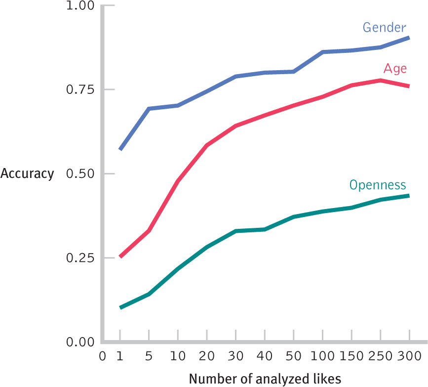
In your own words, what story is this graph telling?
Based on what you learned in Chapter 3 about graphs, explain why the x-
axis is misleading, and describe how you would redesign the graph.
Question 15.49
Athletes’ grades, scatterplots, and correlation: At the university level, the stereotype of the “dumb jock” might be strong and ever present; however, a fair amount of research shows that athletes maintain decent grades and competitive graduation rates when compared to nonathletes. Let’s play with some data to explore the relation between grade point average (GPA) and participation in athletics. Data are presented here for a hypothetical basketball team, including the GPA on a scale of 0.00 to 4.00 for each athlete and the average number of minutes played per game.
| Minutes | GPA |
|---|---|
| 29.70 | 3.20 |
| 32.14 | 2.88 |
| 32.72 | 2.78 |
| 21.76 | 3.18 |
| 18.56 | 3.46 |
| 16.23 | 2.12 |
| 11.80 | 2.36 |
| 6.88 | 2.89 |
| 6.38 | 2.24 |
| 15.83 | 3.35 |
| 2.50 | 3.00 |
| 4.17 | 2.18 |
| 16.36 | 3.50 |
Create a scatterplot of these data and describe your impression of the relation between these variables based on the scatterplot.
Compute the Pearson correlation coefficient for these data.
Explain why the correlation coefficient you just computed is a descriptive statistic, not an inferential statistic. What would you need to do to make this an inferential statistic?
Perform the six steps of hypothesis testing.
What limitations are there to the conclusions you can draw based on this correlation?
How else could you have studied this phenomenon such that you might have been able to draw a more sound, causal conclusion?
Question 15.50
Romantic love, brain activation, and reliability: Aron and colleagues (2005) found a correlation between intense romantic love [as assessed by the Passionate Love Scale (PLS)] and activation in a specific region of the brain [as assessed by functional magnetic resonance imaging (fMRI)]. The PLS (Hatfield & Sprecher, 1986) assessed the intensity of romantic love by asking people in romantic relationships to respond to a series of questions, such as “I want ______ physically, emotionally, and mentally” and “Sometimes I can’t control my thoughts; they are obsessively on ______,” replacing the blanks with the name of their partner.
418
How might we examine the reliability of this measure using test–
retest reliability techniques? Be specific and explain the role of correlation. Would test–
retest reliability be appropriate for this measure? That is, is there likely to be a practice effect? Explain. How could we examine the reliability of this measure using coefficient alpha? Be specific and explain the role of correlation.
Coefficient alpha in this study was 0.81. Based on coefficient alpha, was the use of this scale in this study warranted? Explain.
What is the idea that this measure is trying to assess?
What would it mean for this measure to be valid? Be specific.
Question 15.51
A biased exam question, validity, and correlation: New York State’s fourth-
This test item was supposed to evaluate writing skill. According to the Web site, test items should lead to good student writing; be unambiguous; test for writing, not another skill; and allow for objective, reliable scoring. If students were marked down for talking about the rooster rather than the cow, as alleged by the Web site, would it meet these criteria? Explain. Does this seem to be a valid question? Explain.
The Web site states that New York City schools use the tests to, among other things, evaluate teachers and principals. The logic behind this, ostensibly, is that good teachers and administrators cause higher test performance. List at least two possible third variables that might lead to better performance in some schools than in other schools, other than the presence of good teachers and administrators.
Question 15.52
Holiday weight gain, reliability, and validity: The Wall Street Journal reported on a study of holiday weight gain. Researchers assessed weight gain by asking people how much weight they typically gain in the fall and winter (Parker-
Is the method of asking people about their weight gain likely to be reliable? Explain.
Is this method of asking people about their weight gain likely to be valid? Explain.
Putting It All Together
Question 15.53
Health care spending, longevity, and correlation: New York Times columnist Paul Krugman (2006) used the idea of correlation in a newspaper column when he asked, “Is being an American bad for your health?” Krugman explained that the United States has higher per capita spending on health care than any country in the world and yet is surpassed by many countries in life expectancy (Krugman cited a study by Banks, Marmot, Oldfield, and Smith (2006), published in the Journal of the American Medical Association).
Name the “participants” in this study.
What are the two scale variables being studied, and how was each of them operationalized? Suggest at least one alternate way, other than life expectancy, to operationalize health.
What was the study finding, and why might this finding be surprising? If the finding described above holds true across countries, would this be a negative correlation or a positive correlation? Explain.
Some people thought race or income might be a third variable related to higher spending and lower life expectancy. But Krugman further reported that a comparison of non-
Hispanic white people from America and from England (thus taking race out of the equation) yielded a surprising finding: The wealthiest third of Americans have poorer health than do even the least wealthy third of the English. What are some other possible third variables that might affect both of the variables in this study? Why is this research considered a correlational study rather than a true experiment?
Why would it not be possible to conduct a true experiment to determine whether the amount of health care spending causes changes in health?
Question 15.54
Availability of food, amount eaten, and correlation: Did you know that sometimes you eat more just because the food is in front of you? Geier, Rozin, and Doros (2006) studied how portion size affected the amount people consumed. They discovered interesting things such as that people eat more M&M’s when the candies are dispensed using a big spoon as compared with when a small spoon is used. They investigated whether people eat more when more food is available. Hypothetical data are presented below for the amount of candy presented in a bowl for customers to take and the amount of candy taken by the end of each day of the study:
419
| Number of Pieces Presented | Number of Pieces Taken |
|---|---|
| 10 | 3 |
| 25 | 14 |
| 50 | 26 |
| 75 | 44 |
| 100 | 36 |
| 125 | 57 |
| 150 | 41 |
Create a scatterplot of these data.
Describe your impression of the relation between these variables based on the scatterplot.
Compute the Pearson correlation coefficient for these data.
Summarize your findings using Cohen’s guidelines.
Perform the remaining steps of hypothesis testing.
What limitations are there to the conclusions you can draw based on this correlation?
Use the A-
B- C model to explain possible causes for the relation between these variables.
Question 15.55
High school athletic participation and correlation: Researchers examined longitudinal data to explore the long-
How might high school athletic participation be operationalized as a nominal variable? Be specific.
How might high school athletic participation be operationalized as a scale variable? Be specific.
Why might correlation be a useful tool with data like those used in this study? (Assume the use of scale variables.)
List at least two positive correlations reported by the researchers. Explain why these are positive correlations.
List at least two negative correlations reported by the researchers. Explain why these are negative correlations.
Use the A-
B- C model to offer three different causal explanations for the correlation between high school athletic participation and positive health behaviors. Why might partial correlation be useful in this study? Give at least one specific example of how it might be useful.
Question 15.56
Mental health and partial correlation: A study by Nolan and colleagues (2003) examined the relation between externalizing behaviors (acting out) and anxiety in adolescents. Depression has been shown to relate to both of these variables. What role might depression play in the observed positive relation between these variables? The correlation matrix below displays the Pearson correlation coefficients, as calculated by computer software, for each pair of the variables of interest: depression, externalizing, and anxiety. The Pearson correlation coefficients for each pair of variables are at the intersection in the chart of the two variables. For example, the correlation coefficient for the association between depression (top row) and externalizing (second column of correlations) is 0.635, a very strong positive correlation.
| Correlations | |||
|---|---|---|---|
| Depression | Externalizing | Anxiety | |
| Depression | |||
| Pearson Correlation | 1 | 0.635(**) | 0.368(**) |
| Sig. (2- |
.000 | .000 | |
| N | 220 | 219 | 207 |
| Externalizing | |||
| Pearson Correlation | 0.635(**) | 1 | 0.356(**) |
| Sig. (2- |
.000 | .000 | |
| N | 219 | 220 | 207 |
| Anxiety | |||
| Pearson Correlation | 0.368(**) | 0.356(**) | 1 |
| Sig. (2- |
.000 | .000 | |
| N | 207 | 207 | 207 |
**Correlation is significant at the 0.01 level (2-
420
Given that the authors calculated correlation coefficients, what kind of variables are depression, anxiety, and externalizing? Explain your answer.
What is the correlation coefficient for the association between depression and anxiety? Explain what this correlation coefficient tells us about the relation between these variables.
What is the correlation coefficient for the association between anxiety and externalizing? Explain what this correlation coefficient tells us about the relation between these variables.
The partial correlation of anxiety and externalizing is 0.17, controlling for the variable of depression. How is this different from the original Pearson correlation coefficient between these two variables?
Why is the partial correlation coefficient different from the original Pearson correlation coefficient between these two variables? What did we learn by calculating a partial correlation?
Why can we not draw causal conclusions with respect to these findings?