16.1 Simple Linear Regression
Correlation is a marvelous tool that allows us to know the direction and strength of a relation between two variables. We can also use a correlation coefficient to develop a prediction tool—an equation to predict a person’s score on a scale dependent variable from his or her score on a scale independent variable. For instance, the research team at Michigan State could predict a high score on a measure of social capital for a student who spends a lot of time on Facebook.
Being able to predict the future is powerful stuff and statistical prediction is how it really happens—
423
Prediction versus Relation
Simple linear regression is a statistical tool that lets us predict a person’s score on the dependent variable from his or her score on one independent variable.
The name for the prediction tool that we’ve been discussing is regression, a statistical technique that can provide specific quantitative information that predicts relations between variables. More specifically, simple linear regression is a statistical tool that lets us predict a person’s score on a dependent variable from his or her score on one independent variable.

Simple linear regression allows us to calculate the equation for a straight line that describes the data. Once we can graph that line, we can look at any point on the x-axis and find its corresponding point on the y-axis. That corresponding point is what we predict for y. (Note: As with the Pearson correlation coefficient, we are not able to use simple linear regression if the data do not form the pattern of a straight line.) Let’s consider an example of research that uses regression techniques, and then walk through the steps to develop a regression equation.
Christopher Ruhm, an economist, often uses regression in his research. In one study, he wanted to explore the reasons for his finding (Ruhm, 2000) that the death rate decreases when unemployment goes up—
To explore the reasons for this surprising finding, Ruhm (2006) conducted regression analyses for independent variables related to health (smoking, obesity, and physical activity) and dependent variables related to the economy (income, unemployment, and the length of the workweek). He analyzed data from a sample of nearly 1.5 million participants collected from telephone surveys between 1987 and 2000. Among other things, Ruhm found that a decrease in working hours predicted decreases in smoking, obesity, and physical inactivity.
MASTERING THE CONCEPT
16.1: Simple linear regression allows us to determine an equation for a straight line that predicts a person’s score on a dependent variable from his or her score on the independent variable. We can only use it when the data are approximately linearly related.
424
Regression can take us a step beyond correlation. Regression can provide specific quantitative predictions that more precisely explain relations among variables. For example, Ruhm reported that a decrease in the workweek of just 1 hour predicted a 1% decrease in physical inactivity. Ruhm suggested that shorter working hours free up time for physical activity—
Regression with z Scores
In Chapter 15, we calculated a Pearson correlation coefficient to quantify the relation between students’ numbers of absences from statistics class and their statistics final exam grades; the data for the 10 students in the sample are shown in Table 16-1. Remember, the mean number of absences was 3.400; the standard deviation for these data is 2.375. The mean exam grade was 76.000; the standard deviation for these data is 15.040. The Pearson correlation coefficient that we calculated in Chapter 15 was −0.85, but simple linear regression can take us a step further. We can develop an equation to predict students’ final exam grades from their numbers of absences.
| Student | Absences | Exam Grade |
|---|---|---|
| 1 | 4 | 82 |
| 2 | 2 | 98 |
| 3 | 2 | 76 |
| 4 | 3 | 68 |
| 5 | 1 | 84 |
| 6 | 0 | 99 |
| 7 | 4 | 67 |
| 8 | 8 | 58 |
| 9 | 7 | 50 |
| 10 | 3 | 78 |
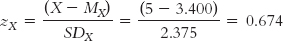
Let’s say that a student (let’s call him Skip) announces on the first day of class that he intends to skip five classes during the semester. We can refer to the size and direction of the correlation (−0.85) as a benchmark to predict his final exam grade. To predict his grade, we unite regression with a statistic we are more familiar with: z scores. If we know Skip’s z score on one variable, we can multiply by the correlation coefficient to calculate his predicted z score on the second variable. Remember that z scores indicate how far a participant falls from the mean in terms of standard deviations. The formula, called the standardized regression equation because it uses z scores, is:
MASTERING THE FORMULA
16- .
.
The subscripts in the formula indicate that the first z score is for the dependent variable, Y, and that the second z score is for the independent variable, X. The ˆ symbol over the subscript Y, called a “hat” by statisticians, refers to the fact that this variable is predicted. This is the z score for “Y hat”—the z score for the predicted score on the dependent variable, not the actual score. We cannot, of course, predict the actual score, and the “hat” reminds us of this. When we refer to this score, we can either say “the predicted score for Y” (with no hat, because we have specified with words that it is predicted) or we can use the hat,  , to indicate that it is predicted. (We would not use both expressions because that would be redundant.) The subscripts X and Y for the Pearson correlation coefficient, r, indicate that this is the correlation between variables X and Y.
425
EXAMPLE 16.1
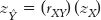
If Skip’s projected number of absences were identical to the mean number of absences for the entire class, then he’d have a z score of 0. If we multiply that by the correlation coefficient, then he’d have a predicted z score of 0 for final exam grade:
So if Skip’s score is right at the mean on the independent variable, then we’d predict that he’d be right at the mean on the dependent variable.
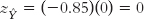
If Skip missed more classes than average and had a z score of 1.0 on the independent variable (1 standard deviation above the mean), then his predicted score on the dependent variable would be −0.85 (that is, 0.85 standard deviation below the mean):
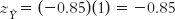
If his z score were −2 (that is, if it were 2 standard deviations below the mean), his predicted z score on the dependent variable would be 1.7 (that is, 1.7 standard deviations above the mean):
Notice two things: First, because this is a negative correlation, a score above the mean on absences predicts a score below the mean on grade, and vice versa. Second, the predicted z score on the dependent variable is closer to its mean than is the z score for the independent variable. Table 16-2 illustrates this for several z scores.
| z Score for the Independent Variable, X | Predicted z Score for the Dependent Variable, Y |
|---|---|
| −2.0 | 1.70 |
| −1.0 | 0.85 |
| 0.0 | 0.00 |
| 1.0 | −0.85 |
| 2.0 | −1.70 |
Regression to the mean is the tendency of scores that are particularly high or low to drift toward the mean over time.
This regressing of the dependent variable—
In the social sciences, many phenomena demonstrate regression to the mean. For example, parents who are very tall tend to have children who are somewhat shorter than they are, although probably still above average. And parents who are very short tend to have children who are somewhat taller than they are, although probably still below average. We explore this concept in more detail later in this chapter.
426
When we don’t have a person’s z score on the independent variable, we have to perform the additional step of converting his or her raw score to a z score. In addition, when we calculate a predicted z score on the dependent variable, we can use the formula that determines a raw score from a z score. Let’s try it with the skipping class and exam grade example, using Skip as the subject.
EXAMPLE 16.2
We already know that Skip has announced his plans to skip five classes. What would we predict for his final exam grade?
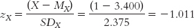
STEP 1: Calculate the z score.
We first have to calculate Skip’s z score on number of absences. Using the mean (3.400) and the standard deviation (2.375) that we calculated in Chapter 15, we calculate:
STEP 2: Multiply the z score by the correlation coefficient.
We multiply this z score by the correlation coefficient to get his predicted z score on the dependent variable, final exam grade:

STEP 3: Convert the z score to a raw score.
We convert from the predicted z score on Y, −0.573, to a predicted raw score for Y:

If Skip skipped five classes, this number would reflect more classes than the typical student skipped, so we would expect him to earn a lower-
The admissions counselor, the insurance salesperson, and Mark Zuckerberg of Facebook, however, are unlikely to have the time or interest to do conversions from raw scores to z scores and back. So the z score regression equation is not useful in a practical sense for situations in which we must make ongoing predictions using the same variables. It is very useful, however, as a tool to help us develop a regression equation we can use with raw scores, a procedure we look at in the next section.
Determining the Regression Equation
You may remember the equation for a line that you learned in geometry class. The version you likely learned was: y = m(x) + b. (In this equation, b is the intercept and m is the slope.) In statistics, we use a slightly different version of this formula:
MASTERING THE FORMULA
16-
= a + b(X) In this formula, X is the raw score on the independent variable and
is the predicted raw score on the dependent variable. a is the intercept of the line, and b is its slope.

The intercept is the predicted value for Y when X is equal to 0, which is the point at which the line crosses, or intercepts, the y-axis.
The slope is the amount that Y is predicted to increase for an increase of 1 in X.
In the regression formula, a is the intercept, the predicted value for Y when X is equal to 0, which is the point at which the line crosses, or intercepts, the y-
= 5 + 2(X). If the score on X is 6, for example, the predicted score for Y is:
= 5 + 2(6) = 5 + 12 = 17. We can verify this on the line in Figure 16-1. Here, we were given the regression equation and regression line, but usually we have to determine these from the data. In this section, we learn the process of calculating a regression equation from data.
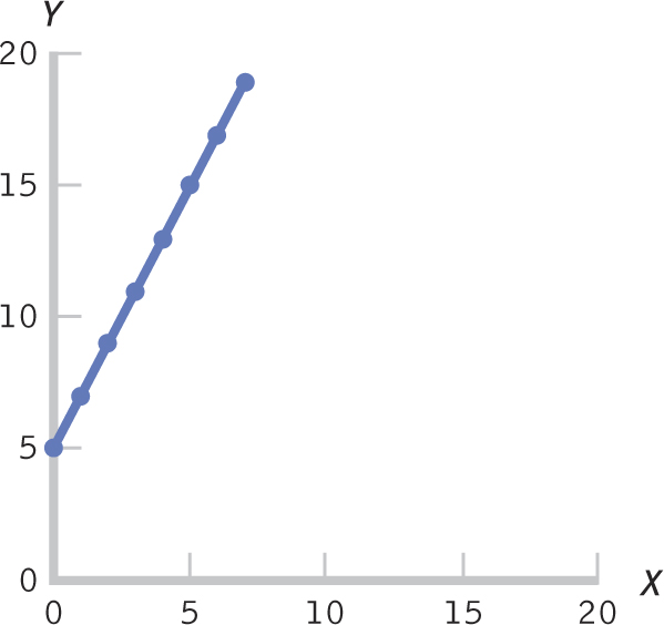
Figure 16-
increases for an increase of 1 in X. Here, the slope is 2. The equation, therefore, is:
= 5 + 2(X).427
Once we have the equation for a line, it’s easy to input any value for X to determine the predicted value for Y. Let’s imagine that one of Skip’s classmates, Allie, anticipates two absences this semester. If we had a regression equation, then we could input Allie’s score of 2 on X and find her predicted score on Y. But first we have to develop the regression equation. Using the z score regression equation to find the intercept and slope enables us to “see” where these numbers come from in a way that makes sense (Aron & Aron, 2002). For this, we use the z score regression equation:  .
.
EXAMPLE 16.3
We start by calculating a, the intercept, a process that takes three steps.
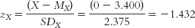
STEP 1: Find the z score for an X of 0.
We know that the intercept is the point at which the line crosses the y-axis when X is equal to 0. So we start by finding the z score for an X of 0 using the formula: 
STEP 2: Use the z score regression equation to calculate the predicted z score on Y.
We use the z score regression equation,  , to calculate the predicted z score on Y for an X of 0.

STEP 3: Convert the z score to its raw score.
We convert the z score for
to its raw score using the formula: 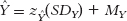 .
.

We have the intercept! When X is 0,
is 94.30. That is, we would predict that someone who never misses class would earn a final exam grade of 94.30.
EXAMPLE 16.4
Next, we calculate b, the slope, a process that is similar to the one for calculating the intercept, but calculating the slope takes four steps. We know that the slope is the amount that
increases when X increases by 1. So all we need to do is calculate what we would predict for an X of 1. We can then compare the
for an X of 0 to the
for an X of 1. The difference between the two is the slope.
STEP 1: Find the z score for an X of 1.
We find the z score for an X of 1, using the formula: 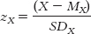
428
STEP 2: Use the z score regression equation to calculate the predicted z score on Y.
We use the z score regression equation,  , to calculate the predicted z score on Y for an X of 1.

STEP 3: Convert the z score to its raw score.
We convert the z score for
to its raw score, using the formula: 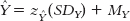 .
.

DETERMINE THE SLOPE.
The prediction is that a student who misses one class would have a final exam grade of 88.919. As X, number of absences, increased from 0 to 1, what happened to
? First, ask yourself if it increased or decreased. An increase would mean a positive slope, and a decrease would mean a negative slope. Here, we see a decrease in exam grade as the number of absences increased. Next, determine how much it increased or decreased. In this case, the decrease is 5.385 (calculated as 94.304 − 88.919 = 5.385). So the slope here is −5.39.
We now have the intercept and the slope and can put them into the equation:
= a + b(X), which becomes
= 94.30 − 5.39(X). We can use this equation to predict Allie’s final exam grade based on her number of absences, two.

Based on the data from our statistics classes, we predict that Allie would earn a final exam grade of 83.52 if she skips two classes. We could have predicted this same grade for Allie using the z score regression equation. The difference is that now we can input any score into the raw-
We can also use the regression equation to draw the regression line and get a visual sense of what it looks like. We do this by calculating at least two points on the regression line, usually for one low score on X and one high score on X. We would always have
for two scores, 0 and 1 (although in some cases these numbers won’t make sense, such as for the variable of human body temperature; you’d never have a temperature that low!). Because these scores are low on the scale for number of absences, we would choose a high score as well; 8 is the highest score in the original data set, so we can use that:

For someone who skipped eight classes, we predict a final exam grade of 51.18. We now have three points, as shown in Table 16-3. It’s useful to have three points because the third point serves as a check on the other two. If the three points do not fall in a straight line, we have made an error.
. Ideally, at least one is low on the scale for X and at least one is high.
| X |
|
|---|---|
| 0 | 94.30 |
| 1 | 88.92 |
| 8 | 51.18 |
We then draw a line through the dots, but it’s not just any line. This line, which you can see in Figure 16-2, is the regression line, which has another name that is wonderfully intuitive: the line of best fit. If you have ever had some clothes tailored to fit your body, perhaps for a wedding or other special occasion, then you know that there really is such a thing as a “best fit.”
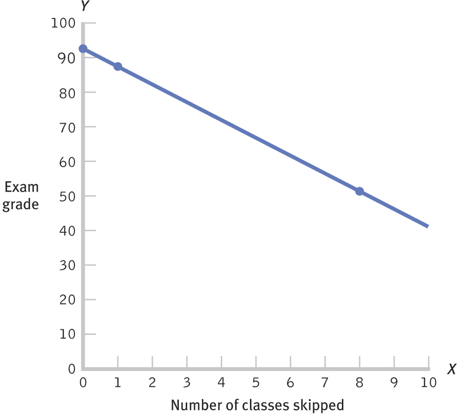
Figure 16-
. We then draw a line through the dots.429
In regression, the meaning of “the line of best fit” is the same as that characteristic in a tailored set of clothes. We couldn’t make the line a little steeper, or raise or lower it, or manipulate it in any way that would make it represent those dots any better than it already does. When we look at the scatterplot around the line in Figure 16-3, we see that the line goes precisely through the middle of the data. Statistically, this is the line that leads to the least amount of error in prediction.
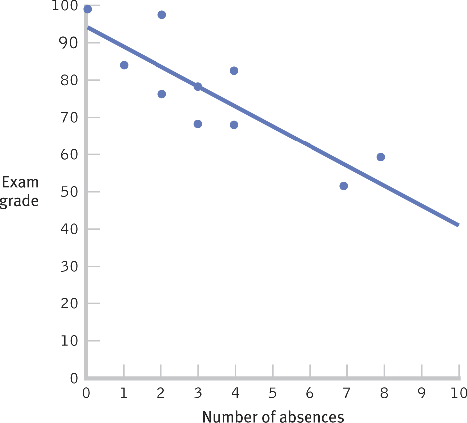
Figure 16-
Language Alert! Notice that the line we just drew starts in the upper left of the graph and ends in the lower right, meaning that it has a negative slope. The word slope is often used when discussing, say, ski slopes. A negative slope means that the line looks like it’s going downhill as we move from left to right. This makes sense because the calculations for the regression equation are based on the correlation coefficient, and the scatterplot associated with a negative correlation coefficient has dots that also go “downhill.” If the slope were positive, the line would start in the lower left of the graph and end in the upper right. A positive slope means that the line looks like it’s going uphill as we move from left to right. Again, this makes sense, because we base the calculations on a positive correlation coefficient, and the scatterplot associated with a positive correlation coefficient has dots that also go “uphill.”
430
The Standardized Regression Coefficient and Hypothesis Testing with Regression
The steepness of the slope tells us the amount that the dependent variable changes as the independent variable increases by 1. So, for the skipping class and exam grades example, the slope of −5.39 tells us that for each additional class skipped, we can predict that the exam grade will be 5.39 points lower. Let’s say that another professor uses skipped classes to predict the class grade on a GPA scale of 0–
The standardized regression coefficient, a standardized version of the slope in a regression equation, is the predicted change in the dependent variable in terms of standard deviations for an increase of 1 standard deviation in the independent variable; symbolized by β and often called beta weight.
This problem might remind you of the problems we faced in comparing scores on different scales. To appropriately compare scores, we standardized them using the z statistic. We can standardize slopes in a similar way by calculating the standardized regression coefficient. The standardized regression coefficient, a standardized version of the slope in a regression equation, is the predicted change in the dependent variable in terms of standard deviations for an increase of 1 standard deviation in the independent variable. It is symbolized by β and is often called a beta weight because of its symbol (pronounced “beta”). It is calculated using the formula:
MASTERING THE FORMULA
16- .
.

We calculated the slope, −5.39, earlier in this chapter. We calculated the sums of squares in Chapter 15. Table 16-4 repeats part of the calculations for the denominator of the correlation coefficient equation. At the bottom of the table, we can see that the sum of squares for the independent variable of classes skipped is 56.4 and the sum of squares for the dependent variable of exam grade is 2262. By inputting these numbers into the formula, we calculate:

| Absences (X) | (X − MX) | (X − MX)2 | Exam Grade (Y) | (Y − MY) | (Y − MY)2 |
|---|---|---|---|---|---|
| 4 | 0.6 | 0.36 | 82 | 6 | 36 |
| 2 | −1.4 | 1.96 | 98 | 22 | 484 |
| 2 | −1.4 | 1.96 | 76 | 0 | 0 |
| 3 | −0.4 | 0.16 | 68 | −8 | 64 |
| 1 | −2.4 | 5.76 | 84 | 8 | 64 |
| 0 | −3.4 | 11.56 | 99 | 23 | 529 |
| 4 | 0.6 | 0.36 | 67 | −9 | 81 |
| 8 | 4.6 | 21.16 | 58 | −18 | 324 |
| 7 | 3.6 | 12.96 | 50 | −26 | 676 |
| 3 | −0.4 | 0.16 | 78 | 2 | 4 |
| ∑(X − MX)2 = 56.4 ∑ (Y − MY)2 = 2262 | |||||
431
Notice that this result is the same as the Pearson correlation coefficient of −0.85. In fact, for simple linear regression, it is always exactly the same. Any difference would be due to rounding decisions for both calculations. Both the standardized regression coefficient and the correlation coefficient indicate the change in standard deviation that we expect when the independent variable increases by 1 standard deviation. Note that the correlation coefficient is not the same as the standardized regression coefficient when an equation includes more than one independent variable, a situation we’ll encounter later in the section “Multiple Regression.”
Because the standardized regression coefficient is the same as the correlation coefficient with simple linear regression, the outcome of hypothesis testing is also identical. The hypothesis-
MASTERING THE CONCEPT
16.2: A standardized regression coefficient is the standardized version of a slope, much like a z statistic is a standardized version of a raw score. For simple linear regression, the standardized regression coefficient is identical to the correlation coefficient. This means that when we conduct hypothesis testing and conclude that a correlation coefficient is statistically significantly different from 0, we can draw the same conclusion about the standardized regression coefficient.
CHECK YOUR LEARNING
Reviewing the Concepts
- Regression builds on correlation, enabling us not only to quantify the relation between two variables but also to predict a score on a dependent variable from a score on an independent variable.
- With the standardized regression equation, we simply multiply a person’s z score on an independent variable by the Pearson correlation coefficient to predict that person’s z score on a dependent variable.
- The raw-
score regression equation is easier to use in that the equation itself does the transformations from raw score to z score and back. - We use the standardized regression equation to build the regression equation that can predict a raw score on a dependent variable from a raw score on an independent variable.
- We can graph the regression line,
= a + b(X), based on values for the y intercept, a; the predicted value on Y when X is 0; and the slope, b, which is the change in Y expected for a 1-
unit increase in X. - The slope, which captures the nature of the relation between the variables, can be standardized by calculating the standardized regression coefficient. The standardized regression coefficient tells us the predicted change in the dependent variable in terms of standard deviations for every increase of 1 standard deviation in the independent variable.
- With simple linear regression, the standardized regression coefficient is identical to the Pearson correlation coefficient.
Clarifying the Concepts
- 16-
1 What is simple linear regression? - 16-
2 What purpose does the regression line serve?
432
Calculating the Statistics
- 16-
3 Let’s assume we know that women’s heights and weights are correlated and the Pearson coefficient is 0.28. Let’s also assume that we know the following descriptive statistics: For women’s height, the mean is 5 feet 4 inches (64 inches), with a standard deviation of 2 inches; for women’s weight, the mean is 155 pounds, with a standard deviation of 15 pounds. Sarah is 5 feet 7 inches tall. How much would you predict she weighs? To answer this question, complete the following steps:- Transform the raw score for the independent variable into a z score.
- Calculate the predicted z score for the dependent variable.
- Transform the z score for the dependent variable back into a predicted raw score.
- 16-
4 Given the regression line
= 12 + 0.67(X), make predictions for each of the following:- X = 78
- X = −14
- X = 52
Applying the Concepts
- 16-
5 In Exercise 15.49, we explored the relation between athletic participation, measured by average minutes played by players on a basketball team, and academic achievement, as measured by GPA. We computed a correlation of 0.344 between these variables. The original, fictional data are presented below. The regression equation for these data is:
= 2.586 + 0.016(X).Minutes GPA 29.70 3.20 32.14 2.88 32.72 2.78 21.76 3.18 18.56 3.46 16.23 2.12 11.80 2.36 6.88 2.89 6.38 2.24 15.83 3.35 2.50 3.00 4.17 2.18 16.36 3.50 - Interpret both the y intercept and the slope in this regression equation.
- Compute the standardized regression coefficient.
- Explain what a strong correlation means for the predictive ability of the regression line.
- What conclusion would you make if you performed a hypothesis test for this regression?
Solutions to these Check Your Learning questions can be found in Appendix D.