Chapter 17 How it Works
17.1 Conducting A Chi-Square Test for Goodness of Fit
Gary Steinman (2006), an obstetrician and gynecologist, studied whether a woman’s diet could affect the likelihood that she would have twins. Insulin-
- Population 1: Vegans who recently gave birth, like those whom we observed. Population 2: Vegans who recently gave birth who are like the general population of mostly nonvegans.
The comparison distribution is a chi-
square distribution. The hypothesis test will be a chi- square test for goodness of fit because we have one nominal variable only. This study meets three of the four assumptions: (1) The one variable is nominal. (2) Every participant is in only one cell (a vegan woman is not counted as having twins and as having one child, or singleton). (3) There are far more than five times as many participants as cells (there are 1042 participants and only two cells). (4) The participants were not, however, randomly selected. We learn from the published research paper that participants were recruited with the assistance of “various vegan societies.” This limits our ability to generalize beyond vegan women like those in the sample. - Null hypothesis: Vegan women give birth to twins at the same rate as the general population. Research hypothesis: Vegan women give birth to twins at a different rate than the general population.
- The comparison distribution is a chi-
square distribution that has 1 degree of freedom: dfχ2 = 2 − 1 = 1. - The critical chi-
square value, based on a p level of 0.05 and 1 degree of freedom, is 3.841, as seen in the curve in Figure 17-3. - Observed (among vegan mothers)
Singleton Twins 1038 4 Expected (based on the 1.9% rate in the general population)
Singleton Twins 1022.202 19.798 Category Observed (O) Expected (E) O − E (O − E)2 
Singleton 1038 1022.202 15.798 249.577 0.244 Twins 4 19.798 −15.798 249.577 12.606 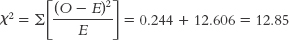
- Reject the null hypothesis; it appears that vegan mothers are less likely to have twins than are mothers in the general population.
The statistics, as reported in a journal article, would read:
χ2 (1, N = 1042) = 12.85, p < 0.05
17.2 Conducting A Chi-Square Test for Independence
Do people who move far from their hometown have a more exciting life? Since 1972, the General Social Survey (GSS) has asked approximately 40,000 adults in the United States numerous questions about their lives. During several years of the GSS, participants were asked, “In general, do you find life exciting, pretty routine, or dull?” (a variable called LIFE) and “When you were 16 years old, were you living in the same (city/town/country)?” (a variable called MOBILE16). How can we use these data to conduct the six steps of hypothesis testing for a chi-
In this case, there are two nominal variables. The independent variable is where a person lives relative to when he or she was 16 years old (same city, same state but different city, different state). The dependent variable is how the person finds life (exciting, routine, dull). Here are the data:
| Exciting | Routine | Dull | |
|---|---|---|---|
| Same city | 4890 | 6010 | 637 |
| Same state/different city | 3368 | 3488 | 337 |
| Different state | 4604 | 4139 | 434 |
- Population 1: People like those in this sample. Population 2: People from a population in which a person’s characterization of life as exciting, routine, or dull does not depend on where that person is living relative to when he or she was 16 years old.
The comparison distribution is a chi-
square distribution. The hypothesis test will be a chi- square test for independence because we have two nominal variables. This study meets all four assumptions: (1) The two variables are nominal. (2) Every participant is in only one cell. (3) There are more than five times as many participants as there are cells (there are 27,907 participants and 9 cells). (4) The GSS sample uses a form of random selection. - Null hypothesis: The proportion of people who find life to be exciting, routine, or dull does not depend on where they live relative to where they lived when they were 16 years old. Research hypothesis: The proportion of people who find life exciting, routine, or dull differs depending on where they live relative to where they lived when they were 16 years old.
- The comparison distribution is a chi-
square distribution with 4 degrees of freedom: dfχ2 = (krow − 1)(kcolumn − 1) = (3 − 1)(3 − 1) = (2)(2) = 4 - The critical chi-
square statistic, based on a p level of 0.05 and 4 degrees of freedom, is 9.488. 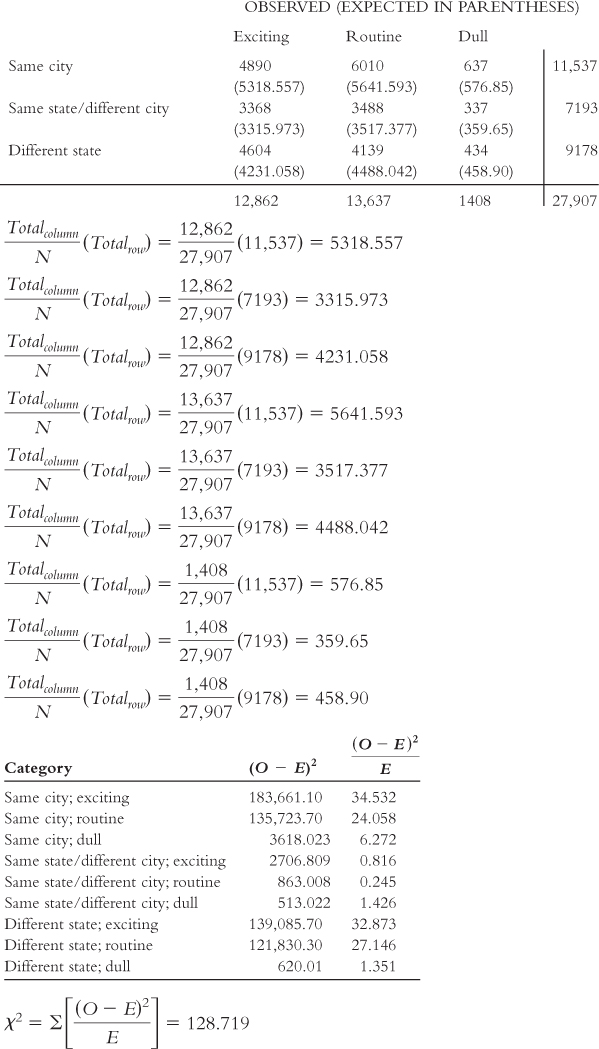
- Reject the null hypothesis. The calculated chi-
square statistic exceeds the critical value. How exciting a person finds life does appear to vary with where the person lives relative to where he or she lived when he or she was 16 years old. We would present these statistics in a journal article as: χ2 (4, N = 27,907) = 128.72, p < 0.05
17.3 Calculating Cramer’s V
What is the effect size, Cramer’s V, for the chi-
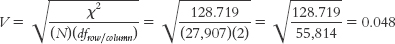
According to Cohen’s conventions, this is a small effect size. With this piece of information, we’d present the statistics in a journal article as:
χ2 (4, N = 27,907) = 128.72, p < 0.05, Cramer‘s V = 0.05