Chapter 17 Exercises
Clarifying the Concepts
Question 17.1
Distinguish nominal, ordinal, and scale data.
Question 17.2
What are the three main situations in which we use a nonparametric test?
Question 17.3
What is the difference between the chi-
Question 17.4
What are the four assumptions for the chi-
Question 17.5
List two ways in which statisticians use the word independence or independent with respect to concepts introduced earlier in this book. Then describe how independence is used by statisticians with respect to chi square.
Question 17.6
What are the hypotheses when conducting the chi-
Question 17.7
How are the degrees of freedom for the chi-
Question 17.8
Why is there just one critical value for a chi-
Question 17.9
What information is presented in a contingency table in the chi-
Question 17.10
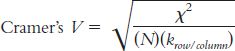
What measure of effect size is used with chi square?
Question 17.11
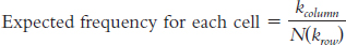
Define the symbols in the following formula: 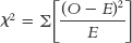
.
Question 17.12
What is the formula 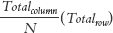
used for?
Question 17.13
What information does the measure of relative likelihood provide?
Question 17.14
In order to calculate relative likelihood, what must we first calculate?
Question 17.15
What is the difference between relative likelihood and relative risk?
Question 17.16
Why might relative likelihood be easier to understand as an effect size than Cramer’s V?
Question 17.17
Which graph is most useful for displaying the results of a chi-
Question 17.18
How are adjusted standardized residuals calculated?
Question 17.19
How are adjusted standardized residuals used as a post hoc test for chi-
Calculating the Statistics
Question 17.20
For each of the following, (i) identify the incorrect symbol, (ii) state what the correct symbol should be, and (iii) explain why the initial symbol was incorrect.
For the chi-
square test for goodness of fit: dfχ2 = N − 1 For the chi-
square test for independence: dfχ2 = (krow − 1) + (kcolumn − 1) 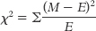
Question 17.21
For each of the following, identify the independent variable(s), the dependent variable(s), and the level of measurement (nominal, ordinal, scale).
The number of loads of laundry washed per month was tracked for women and men living in college dorms.
A researcher interested in people’s need to maintain social image collected data on the number of miles on someone’s car and his or her rank for “need for approval” out of the 183 people studied.
A professor of social science was interested in whether involvement in campus life is significantly impacted by whether a student lives on or off campus. Thirty-
seven students living on campus and 37 students living off campus were asked whether they were an active member of a club.
Question 17.22
Use this calculation table for the chi-
| Category | Observed (O) | Expected (E) | O − E | (O − E)2 |

|
|---|---|---|---|---|---|
| 1 | 48 | 60 | |||
| 2 | 46 | 30 | |||
| 3 | 6 | 10 |
Calculate degrees of freedom for this chi-
square test for goodness of fit. Perform all of the calculations to complete this table.
Compute the chi-
square statistic.
Question 17.23
Use this calculation table for the chi-
| Category | Observed (O) | Expected (E) | O − E | (O − E)2 |

|
|---|---|---|---|---|---|
| 1 | 750 | 625 | |||
| 2 | 650 | 625 | |||
| 3 | 600 | 625 | |||
| 4 | 500 | 625 |
Calculate degrees of freedom for this chi-
square test for goodness of fit. Perform all of the calculations to complete this table.
Compute the chi-
square statistic.
Question 17.24
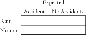
Below are some data to use in a chi-
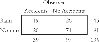
Calculate the degrees of freedom for this test.
Complete this table of expected frequencies.
Calculate the test statistic.
Calculate the appropriate measure of effect size.
Calculate the relative likelihood of accidents, given that it is raining.
Question 17.25
The data below are from a study of lung cancer patients in Turkey (Yilmaz et al., 2000). Use these data to calculate the relative likelihood of being a smoker, given that a person is female rather than male.
| Nonsmoker | Smoker | |
|---|---|---|
| Female | 186 | 13 |
| Male | 182 | 723 |
Question 17.26
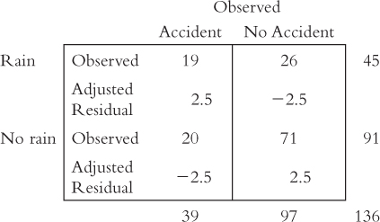
The following table (output from SPSS) represents the observed frequencies for the data presented in Exercise 17.24 and the adjusted standardized residuals for each of the cells. Using this information and the criterion of 2, indicate for which of these cells there is a significant difference between the observed and the expected frequencies.
Applying the Concepts
Question 17.27
Gender, salary negotiation, and chi square: Researchers investigated whether or not language in job postings affected the likelihood that women and men would negotiate regarding salary (Leibbrandt & List, 2012). Some job postings clearly indicated that the salary was negotiable, and others contained no such statement. The postings were otherwise identical. The researchers examined the behavior of almost 2500 applicants for one of the jobs in these advertisements. The graph on the next page shows the proportions of women and men who negotiated in response to either type of listing.
488
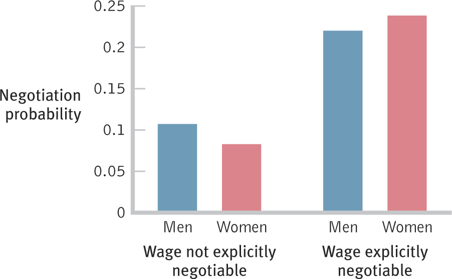
What are the variables in this study, what are their levels, and what types of variables are they?
Explain why the researchers would have been able to use chi square in this study. Which type of chi-
square test would have been appropriate? Based on the graph, explain in your own words what the researchers found.
Question 17.28
Gender, the Oscars, and nonparametric tests: In 2010, Sandra Bullock won an Academy Award for best actress. Shortly thereafter, she discovered that her husband was cheating on her. Headlines erupted about a supposed Oscar curse that befalls women, and many in the media wondered whether ambitious women—
A good researcher always asks, “Compared to what?” In this case, what would be an appropriate comparison group to use to determine whether there really is a gender difference in likelihood of relationship breakups among Oscar winners? Explain your answer.
Kate Harding (2010) reported that many men—
including Russell Crowe, William Hurt, Dustin Hoffman, Robert Duvall, and Clark Gable— experienced the same outcome. Indeed, Harding counted 15 best actor winners, compared with just 8 best actress winners, who divorced not long after winning an Oscar. If she wanted to conduct statistical analyses, what test would Harding use? Explain your answer. Explain how an illusory correlation, bolstered by a confirmation bias, might have led to the headlines despite evidence to the contrary.
Question 17.29
Parametric or nonparametric test? For each of the following research questions, state whether a parametric or nonparametric hypothesis test is more appropriate. Explain your answers.
Are women more or less likely than men to be economics majors?
At a small company with 15 staff and one top boss, do those with a college education tend to make a different amount of money than those without one?
At your high school, did athletes or nonathletes tend to have higher grade point averages?
At your high school, did athletes or nonathletes tend to have higher class ranks?
Compare car accidents in which the occupants were wearing seat belts with accidents in which the occupants were not wearing seat belts. Do seat belts seem to make a difference in the numbers of accidents that lead to no injuries, nonfatal injuries, and fatal injuries?
Compare car accidents in which the occupants were wearing seat belts with accidents in which the occupants were not wearing seat belts. Were those wearing seat belts driving at slower speeds, on average, than those not wearing seat belts?
Question 17.30
Types of variables and student evaluations of professors: Weinberg, Fleisher, and Hashimoto (2007) studied almost 50,000 students’ evaluations of their professors in nearly 400 economics courses at the Ohio State University over a 10-
I—
II—
III—
Explain your answer to part (iii).
The researchers found that students’ ratings of their professors were predictive of grades in the class for which the professor was evaluated.
The researchers also found that students’ ratings of their professors were not predictive of grades for other, related future classes. (The researchers stated that these first two findings suggest that student ratings of professors are tied to their current grades but not to learning—
which would affect future grades.) The researchers found that male professors received statistically significantly higher student ratings, on average, than did female professors.
The researchers reported, however, that average levels of students’ learning (as assessed by grades in related future classes) were not statistically significantly different for those who had male and those who had female professors.
The researchers might have been interested in whether there were proportionally more female professors teaching upper-
level than lower- level courses and proportionally more male professors teaching lower- level than upper- level courses (perhaps a reason for the lower average ratings of female professors). The researchers found no statistically significant differences in average student evaluations among non-
tenure- track lecturers, graduate student teaching associates, and tenure- track faculty members.
Question 17.31
Grade inflation and types of variables: A New York Times article on grade inflation reported several findings related to a tendency for average grades to rise over the years and a tendency for the top-
I—
II—
III—
Explain your answer to part (iii).
In 1969, seven percent of all grades were A’s; in 1994, twenty-
five percent of all grades were A’s. The average GPA for the graduating students of elite schools is 3.2, the average GPA for graduating students at selective schools (the level below elite schools) is 3.04, and the average GPA for graduating students at state colleges is 2.95.
At Dartmouth College, an elite university, SAT scores of incoming students have increased along with their subsequent college GPAs (perhaps an explanation for grade inflation).
Question 17.32
High school academic performance and types of variables: Here are three ways to assess one’s performance in high school: (1) GPA at graduation, (2) whether one graduated with honors (as indicated by graduating with a GPA of at least 3.5), and (3) class rank at graduation. For example, Abdul had a 3.98 GPA, graduated with honors, and was ranked 10th in his class.
Which of these variables could be considered a nominal variable? Explain.
Which of these variables is most clearly an ordinal variable? Explain.
Which of these variables is a scale variable? Explain.
Which of these variables gives us the most information about Abdul’s performance?
If we were to use one of these variables in an analysis, which variable (as the dependent variable) would lead to the lowest chance of a Type II error? Explain why.
Question 17.33
Immigration, crime, and research design: “Do Immigrants Make Us Safer?” asked the title of a New York Times Magazine article (Press, 2006). The article reported findings from several U.S.-based studies, including several conducted by Harvard sociologist Robert Sampson in Chicago. For each of the following findings, draw the table of cells that would comprise the research design. Include the labels for each row and column.
Mexicans were more likely to be married (versus single) than either blacks or whites.
People living in immigrant neighborhoods were 15% less likely than were people living in nonimmigrant neighborhoods to commit crimes. This finding was true among both those living in households headed by a married couple and those living in households not headed by a married couple.
The crime rate was higher among second-
generation than among first- generation immigrants; moreover, the crime rate was higher among third- generation than among second- generation immigrants.
Question 17.34
Sex selection and hypothesis testing: Across all of India, there are only 933 girls for every 1000 boys (Lloyd, 2006), evidence of a bias that leads many parents to illegally select for boys or to kill their infant girls. (Note that this translates into a proportion of girls of 0.483.) In Punjab, a region of India in which residents tend to be more educated than in other regions, there are only 798 girls for every 1000 boys. Assume that you are a researcher interested in whether sex selection is more or less prevalent in educated regions of India, and that 1798 children from Punjab constitute the entire sample. (Hint: You will use the proportions from the national database for comparison.)
How many variables are there in this study? What are the levels of any variable you identified?
Which hypothesis test would be used to analyze these data? Justify your answer.
Conduct the six steps of hypothesis testing for this example. (Note: Be sure to use the correct proportions for the expected values, not the actual numbers for the population.)
Report the statistics as you would in a journal article.
Question 17.35
Gender, op-
How many variables are there in this study? What are the levels of any variable you identified?
Which hypothesis test would be used to analyze these data? Justify your answer.
Conduct the six steps of hypothesis testing for this example.
Report the statistics as you would in a journal article.
490
Question 17.36
Romantic music, behavior, chi square, and effect size: Guéguen, Jacob, and Lamy (2010) investigated whether exposure to romantic music affects dating behavior. The participants, young, single French women, waited for the experiment to start in a room in which songs with either romantic lyrics or neutral lyrics were playing. After a few minutes, each woman who participated completed a marketing survey administered by a young male confederate. During a break, the confederate asked the participant for her phone number. Of the women who listened to romantic music, 52.2% (23 out of 44) gave him her phone number, whereas 27.9% (12 out of 43) of the women who listened to neutral music did so. The researchers conducted a chi-
Calculate Cramer’s V. What size effect is this?
Calculate the relative likelihood of providing her phone number for women listening to romantic music versus neutral music. Explain what we learn from this relative likelihood.
Question 17.37
The General Social Survey, an exciting life, and relative risk: In How It Works 17.2, we walked through a chi-
Construct a table that shows only the appropriate conditional proportions for this example. For example, the percentage of people who find life exciting, given that they live in the same city, is 42.4. The proportion, therefore, is 0.424.
Construct a graph that displays these conditional proportions.
Calculate the relative risk (or relative likelihood) of finding life exciting if one lives in a different state compared to if one lives in the same city as one did at 16.
Question 17.38
Gender, ESPN, and chi square: Many of the numbers we see in the news could be analyzed with chi square. The feminist blog Culturally Disoriented examined the photos in the 2012 “body issue” of ESPN The Magazine—the publication’s annual spread of photographs of nude athletes. The blogger reported: “Female athlete after female athlete was photographed not as a talented, powerful sportswoman, but as…eye candy” (http:/
Why is a chi-
square statistical analysis a good choice for these data? Which kind of chi- square test should you use? Explain your answer. Conduct the six steps of hypothesis testing for this example.
Calculate an effect size. Explain why there might be a fairly substantial effect size even though we were not able to reject the null hypothesis.
Report the statistics as you would in a journal article.
Construct a table that shows only the appropriate conditional proportions for this example—
that is, the proportion of people in active poses given that they are men or women. Construct a graph that displays these conditional proportions.
Calculate the relative likelihood of being photographed in an active pose if you are a male athlete compared to if you are a female athlete.
Question 17.39
Premarital doubts, divorce, and chi square: In an article titled “Do Cold Feet Warn of Trouble Ahead?”, researchers studied 464 married heterosexual spouses to determine whether or not doubts before marriage were predictive of marital troubles, and divorce, later on (Lavner, Karney, & Bradbury, 2012). The following is an excerpt from the results section of their paper: “For husbands, 9% of those who reported not having premarital doubts divorced by four years (n = 10 of 117) compared with 14% of those who did report premarital doubts (n = 15 of 106); these groups did not differ significantly, χ2 (1, n = 223) = 1.76, p > .10. Among wives, 8% of those who reported not having premarital doubts divorced by four years (n = 11 of 141) compared with 19% of those who did report premarital doubts (n = 16 of 84). Chi-
What are the variables in this study, and what are their levels?
Explain why the researchers were able to use chi-
square tests. Which kind of chi- square tests did they use? What changes would the APA want to see in the reporting of these results?
Explain in your own words what the researchers found.
Question 17.40
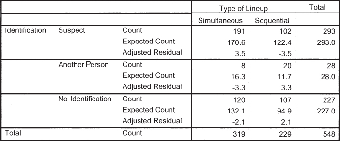
Police lineups, SPSS, and adjusted standardized residual: In Check Your Learning 17-
For simultaneous lineups, what is the observed frequency for the identification of suspects?
For sequential lineups, what is the expected frequency for the identification of a person other than the suspect?
For simultaneous lineups, what is the adjusted standardized residual for cases in which there was no identification? What does this number indicate?
If you were to use an adjusted standardized residual criterion of 2 (regardless of the sign), for which cells would you conclude that the difference between observed frequency and expected frequency is greater than you would expect if the two variables were independent?
Repeat part (d) for an adjusted standardized residual criterion of 3 (regardless of the sign).
Putting It All Together
Question 17.41
Gender bias, poor growth, and hypothesis testing: Grimberg, Kutikov, and Cucchiara (2005) wondered whether gender biases were evident in referrals of children for poor growth. They believed that boys were more likely to be referred even when there was no problem—
How many variables are there in this study? What are the levels of any variable you identified?
Which hypothesis test would be used to analyze these data? Justify your answer.
Conduct the six steps of hypothesis testing for this example.
Calculate the appropriate measure of effect size. According to Cohen’s conventions, what size effect is this?
Report the statistics as you would in a journal article.
Draw a table that includes the conditional proportions for boys and for girls.
Create a graph with bars showing the proportions for all six conditions.
Among only children who are below height norms, calculate the relative risk of having an underlying medical condition if one is a boy as opposed to a girl. Show your calculations.
Explain what we learn from this relative risk.
Now calculate the relative risk of having an underlying medical condition if one is a girl. Show your calculations.
Explain what we learn from this relative risk.
Explain how the calculations in parts (h) and (j) provide us with the same information in two different ways.
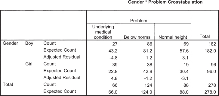
Below is a printout from SPSS software that depicts the data for the six cells. For each cell, there is an observed frequency (count), expected frequency (expected count), and adjusted standardized residual (adjusted residual). For boys, what are the observed and expected frequencies for having an underlying medical condition?
For boys, what is the adjusted standardized residual for those with an underlying medical condition? What does this number indicate? If you used an adjusted standardized residual criterion of 2 (regardless of the sign), for which cells would you conclude that the difference between observed frequency and expected frequency is greater than you would expect if the two variables were independent? What if you used an adjusted standardized residual criterion of 3 (regardless of the sign). Are the results different from those using a criterion of 2? If yes, explain how they’re different.
492
Question 17.42
The prisoner’s dilemma, cross-
| Defect | Cooperate | |
|---|---|---|
| China | 31 | 36 |
| United States | 41 | 14 |
How many variables are there in this study? What are the levels of any variables you identified?
Which hypothesis test would be used to analyze these data? Justify your answer.
Conduct the six steps of hypothesis testing for this example, using the above data.
Calculate the appropriate measure of effect size. According to Cohen’s conventions, what size effect is this?
Report the statistics as you would in a journal article.
Draw a table that includes the conditional proportions for participants from China and from the United States.
Create a graph with bars showing the proportions for all four conditions.
Create a graph with two bars showing just the proportions for the defections for each country.
Calculate the relative risk (or relative likelihood) of defecting, given that one is from China versus the United States. Show your calculations.
Explain what we learn from this relative risk.
Now calculate the relative risk of defecting, given that one is from the United States versus China. Show your calculations.
Explain what we learn from this relative risk.
Explain how the calculations in parts (i) and (k) provide us with the same information in two different ways.