18.2 Nonparametric Hypothesis Tests
We sometimes want to compare groups with respect to a dependent variable that does not meet the criteria for a parametric test. Fortunately, there are several nonparametric hypothesis tests that can be used to answer important research questions—
The Wilcoxon Signed-Rank Test
EXAMPLE 18.3
The Wilcoxon signed-
| Country | 1995– |
2003– |
Difference |
|---|---|---|---|
| United States | 3.11 | 4.00 | 0.89 |
| Australia | 2.10 | 2.90 | 0.80 |
| Ireland | 3.36 | 2.90 | −0.46 |
| New Zealand | 2.62 | 2.60 | −0.02 |
| Canada | 2.56 | 2.40 | −0.16 |
| Great Britain | 2.09 | 2.20 | 0.11 |
503
The Wilcoxon signed-
The independent variable for this analysis is time period, with two levels: 1995–
For nonparametric tests, the six steps of hypothesis testing are similar to those for parametric tests. The good news is that these six steps for nonparametric hypothesis tests are usually easier to compute, and some of the steps, such as the one for assumptions, are shorter. We will outline the six steps for hypothesis testing with the Wilcoxon signed-
STEP 1: Identify the assumptions.
There are three assumptions. (1) The differences between pairs must be able to be ranked. (2) We should use random selection, or the ability to generalize will be limited. (3) The difference scores should come from a symmetric population distribution. This third assumption, combined with the fact that the paired-
Summary: We convert the data from scale to ordinal. The researchers did not indicate whether they used random selection to choose the countries in the sample, so we must be cautious when generalizing from these results. It is difficult to know from a small sample whether the difference scores come from a symmetric population distribution.
504
STEP 2: State the null and research hypotheses.
We state the null and research hypotheses only in words, not in symbols.
Summary: Null hypothesis: English-
STEP 3: Determine the characteristics of the comparison distribution.
We use the Wilcoxon signed-
Summary: We use a p level of 0.05 and a two-
STEP 4: Determine the critical values, or cutoffs.
We use Table B.9 from Appendix B to determine the cutoff, or critical value, for the Wilcoxon signed-
Summary: The cutoff for a Wilcoxon signed-
STEP 5: Calculate the test statistic.
We start the calculations by organizing the difference scores from highest to lowest in terms of absolute value, as seen in Table 18-5. Because we organize by absolute value, −0.46 is higher than 0.11, for example. We then rank the absolute values of the differences, as seen in the second column of numbers in Table 18-5. We separate the ranks into two columns, the fourth and fifth columns in the table. The fourth column includes only the ranks associated with positive differences, and the fifth column includes only the ranks associated with negative differences. (Note: We omit any difference scores of 0 from the ranking and from any further calculations.)
| Country | Difference | Ranks | Ranks for Positive Differences | Ranks for Negative Differences |
|---|---|---|---|---|
| United States | 0.89 | 1 | 1 | |
| Australia | 0.80 | 2 | 2 | |
| Ireland | −0.46 | 3 | 3 | |
| Canada | −0.16 | 4 | 4 | |
| Great Britain | 0.11 | 5 | 5 | |
| New Zealand | −0.02 | 6 | 6 |
Table 18-5 also serves as a graph. We can determine by the pattern of the ranks in the last two columns whether there seems to be a difference. The pattern for these data suggests that there has been more of an increase than a decrease in accomplishment-
The final step in calculating the test statistic is to sum the ranks for the positive scores and, separately, sum the ranks for the negative scores.
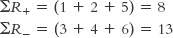
The work is done. The smaller of these is the test statistic, T. The formula is:
MASTERING THE FORMULA
18-
T = ∑Rsmaller
In this case, T = ∑R+ = 8.
505
Summary: T = ∑Rsmaller (Note: Show all calculations in your summary.)
STEP 6: Make a decision.
The test statistic, 8, is not smaller than the critical value, 0, so we fail to reject the null hypothesis. We expected this from the very small critical value. We likely did not have sufficient statistical power to detect any real differences that might exist. We cannot conclude that the two groups are different with respect to accomplishment-
After completing the hypothesis test, we report the primary statistical information in a format similar to that used for parametric tests. In the write-
T = 8, p > 0.05
(Note: If we conduct the Wilcoxon signed-
The Mann–Whitney U Test
The Mann–
As mentioned earlier, most parametric hypothesis tests have nonparametric equivalents. In this section, we learn how to conduct one of the most common of these tests—
MASTERING THE CONCEPT
18.2: We conduct a Mann–
EXAMPLE 18.4
The researchers observed that countries with a recent communist past tended to have lower ranks on national pride (Smith & Kim, 2006). Let’s choose 10 European countries, 5 of which were communist during part of the twentieth century. The independent variable is type of country, with two levels: formerly communist and not formerly communist. The dependent variable is rank on accomplishment-
| Country | Pride Score |
|---|---|
| Noncommunist | |
| Ireland | 2.9 |
| Austria | 2.4 |
| Spain | 1.6 |
| Portugal | 1.6 |
| Sweden | 1.2 |
| Communist | |
| Hungary | 1.6 |
| Czech Republic | 1.3 |
| Slovenia | 1.1 |
| Slovakia | 1.1 |
| Poland | 0.9 |
506
As noted earlier, nonparametric tests use the same six steps of hypothesis testing as parametric tests but are usually easier to calculate.
STEP 1: Identify the assumptions.
There are three assumptions. (1) The data must be ordinal. (2) We should use random selection; otherwise, the ability to generalize will be limited. (3) Ideally, no ranks are tied. The Mann–
Summary: (1) We need to convert the data from scale to ordinal. (2) The researchers did not indicate whether they used random selection to choose the European countries in the sample, so we must be cautious when generalizing from these results. (3) There are some ties, but we will assume that there are not so many as to render the results of the test invalid.
STEP 2: State the null and research hypotheses.
We state the null and research hypotheses only in words, not in symbols.
Summary: Null hypothesis: Formerly communist European countries and European countries that have not been communist do not tend to differ in accomplishment-
STEP 3: Determine the characteristics of the comparison distribution.
The Mann–
507
Summary: There are five countries in the formerly communist group and five countries in the noncommunist group.
STEP 4: Determine the critical values, or cutoffs.
There are two Mann–
Summary: The cutoff, or critical value, for a Mann–
STEP 5: Calculate the test statistic.
As noted above, we calculate two test statistics for a Mann–
| Country | Pride Score | Pride Rank | Type of Country | NC Rank | C Rank |
|---|---|---|---|---|---|
| Ireland | 2.9 | 1 | NC | 1 | |
| Austria | 2.4 | 2 | NC | 2 | |
| Spain | 1.6 | 4 | NC | 4 | |
| Portugal | 1.6 | 4 | NC | 4 | |
| Hungary | 1.6 | 4 | C | 4 | |
| Czech Republic | 1.3 | 6 | C | 6 | |
| Sweden | 1.2 | 7 | NC | 7 | |
| Slovenia | 1.1 | 8.5 | C | 8.5 | |
| Slovakia | 1.1 | 8.5 | C | 8.5 | |
| Poland | 0.9 | 10 | C | 10 |
508
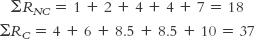
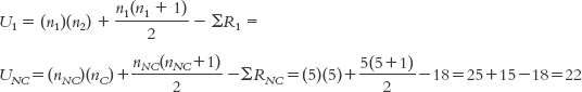
Before we continue, we sum the ranks (R) for each group and add subscripts to indicate which group is which:
The formula for the first group, with the n’s referring to sample size in a particular group, is:
MASTERING THE FORMULA
![]() 18-
18-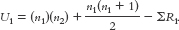 The formula for the second group is:
 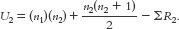 The symbol n refers to the sample size for a particular group. In these formulas, the first group is labeled 1 and the second group is labeled 2. ΣR refers to the sum of the ranks for a particular group.
The formula for the second group is:
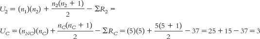
Summary: UNC = 22; UC = 3.
STEP 6: Make a decision.
For a Mann–
Summary: The test statistic, 3, is not smaller than the critical value, 2. We cannot reject the null hypothesis. We conclude only that insufficient evidence exists to show that the two groups are different with respect to accomplishment-
After completing the hypothesis test, we want to present the primary statistical information in a report. In the write-
U = 3, p > 0.05
(Note: If we conduct the Mann–
The Kruskal–Wallis H Test
EXAMPLE 18.5
The Kruskal–
| Asia | Pride | Europe | Pride | South America | Pride |
|---|---|---|---|---|---|
| Japan | 1.80 | Finland | 1.80 | Venezuela | 3.60 |
| South Korea | 1.00 | Portugal | 1.60 | Chile | 2.30 |
| Taiwan | 0.90 | France | 1.50 | Uruguay | 2.00 |
509
The Kruskal–
We want to convert the data from scale to ordinal during the calculations. This is similar to what we did when we used a Mann–
As with the other nonparametric hypothesis tests, we use the same six steps of hypothesis testing.
STEP 1: Identify the assumptions.
There are two assumptions. (1) The data must be ordinal. (2) We should use random selection; otherwise, the ability to generalize will be limited.
Summary: We convert the data from scale to ordinal. The researchers did not indicate whether they used random selection to choose the countries in the sample, so we must be cautious when generalizing from these results.
STEP 2: State the null and research hypotheses.
We will state the null and research hypotheses only in words, not in symbols.
Summary: Null hypothesis: The population distributions for accomplishment-
STEP 3: Determine the characteristics of the comparison distribution.
The Kruskal–
510
Summary: We use the chi-
STEP 4: Determine the critical values, or cutoffs.
We use the chi-
Summary: The cutoff for a Kruskal–
STEP 5: Calculate the test statistic.
We start the calculations by organizing the data by raw score from highest to lowest in one single column, and then by rank in the next column. The scores for Finland and Japan are both 1.8. We deal with this tie by assigning them the average of the two ranks they would hold, 4 and 5. They both receive the average of these ranks, 4.5. We include the group membership of each participant (country) next to its score and rank. A indicates an Asian country; E represents a European country; S represents a South American country. Table 18-9 shows these data.
| Country | Pride Score | Pride Rank | Type of Country | A Ranks | E Ranks | S Ranks |
|---|---|---|---|---|---|---|
| Venezuela | 3.6 | 1 | S | 1 | ||
| Chile | 2.3 | 2 | S | 2 | ||
| Uruguay | 2.0 | 3 | S | 3 | ||
| Finland | 1.8 | 4.5 | E | 4.5 | ||
| Japan | 1.8 | 4.5 | A | 4.5 | ||
| Portugal | 1.6 | 6 | E | 6 | ||
| France | 1.5 | 7 | E | 7 | ||
| South Korea | 1.0 | 8 | A | 8 | ||
| Taiwan | 0.9 | 9 | A | 9 |
The final three columns of Table 18-9 separate the ranks by group. From these columns, we can easily see that the South American countries tend to hold the highest ranks. Of course, we want to conduct the hypothesis test before drawing any conclusions. Notice that the format of this table is the same as that for the Mann–
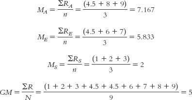
Before we continue, we take the mean of the ranks for each group, including subscripts to indicate which group is which. Notice that we are taking the mean of the ranks, not the sum of the ranks as we did with the Mann–
511
MASTERING THE FORMULA
![]() 18-
18- . We sum the ranks for every participant in that group, then divide by the total number of participants in that group. The formulas for the other groups are the same.
MASTERING THE FORMULA
18- We sum the ranks for every participant in the entire study, then divide by the total number of participants in the entire study.
The formula for the test statistic, H, is:
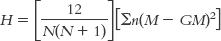
The 12 is a constant; it is always in the equation. The uppercase N’s in the first part of the equation refer to the sample size for the whole study, 9. The lowercase n refers to the sample size for each group. The second part of the equation tells us to make that calculation for each group using its sample size (n), mean rank (M), and the grand mean (GM; the mean rank for the whole study). The summation sign, ∑, tells us that we have to do this calculation for each group and then add them together.
If there were no differences, each group would have the same mean rank, which would be the same as the grand mean. If the mean rank for each group were exactly equal to the grand mean, the second part of the equation would be 0, which, when multiplied by the first part, would still be 0. So an H of 0 indicates no difference among mean ranks. Similarly, as the mean ranks for the individual samples get farther from the grand mean, the second part of the equation becomes larger, and the test statistic is larger.
MASTERING THE FORMULA
18- The 12 is a constant; it is always in the equation. The two N’s refer to the total number of participants in the study. The lowercase n refers to the sample size for each group. M is the mean rank for each group, and GM is the grand mean.
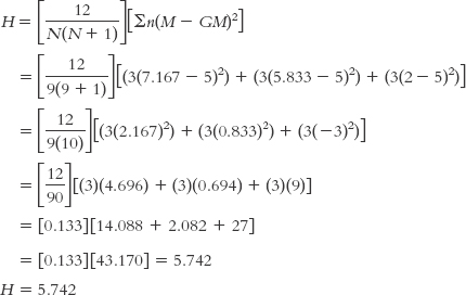
Summary: H = 5.74
512
STEP 6: Make a decision.
For a Kruskal–
Summary: The test statistic, 5.74, is not larger than the critical value, 5.992. We cannot reject the null hypothesis. We can conclude only that there is insufficient evidence that there are differences among the countries based on region.
After completing the hypothesis test, we want to present the primary statistical information in a report. In the write-
H = 5.742, p > 0.05.
(Note: If we conduct the Kruskal–
Next Steps
Bootstrapping
Bootstrapping is a statistical process in which the original sample data are used to represent the entire population, and samples are repeatedly taken from the original sample data to form a confidence interval.
We sometimes describe people as “pulling themselves up by their own bootstraps” when they create personal success with minimal resources. Statisticians borrowed the word when they had to maximize the information they could gain from only a few resources. Bootstrapping is a statistical process in which the original sample data are used to represent the entire population, and samples are repeatedly taken from the original sample data to form a confidence interval.
When bootstrapping data, we use no information other than the sample data. But we treat the sample data as if they constitute the entire population. The secret to successful statistical bootstrapping is one clever technique: sampling with replacement. We first take the mean of the original sample, and then we continue to sample from the original sample. Specifically, we repeatedly take the same number of participants’ scores from the sample (e.g., if there are eight participants in the sample, we keep drawing eight participants’ scores from that pool), as if we’re drawing from the population, and calculate the mean. In bootstrapping, we do this by replacing each participant, one by one, immediately after we select his or her score to be part of the sample.
Here’s an example. If the eight scores are 1, 5, 6, 6, 8, 9, 12, and 13 (with a mean of 7.5), then we would repeatedly pull eight scores, one at a time. But after pulling each single score, we put it back, making it possible to pull that exact same score again—
Table 18-10 shows just a few possible samples from the original sample (all samples are arranged from lowest to highest, although it is unlikely that they would have been drawn in this order). Of course, doing this by hand would take a very long time, particularly with a sample much larger than eight, so we rely on the computer to do the work for us. So now we have the mean of the original sample of eight (which was 7.5) and thousands of means of samples of eight drawn from the original sample—
| Sample | Mean | |||||||
|---|---|---|---|---|---|---|---|---|
| 5 | 6 | 6 | 6 | 8 | 12 | 13 | 13 | 8.625 |
| 1 | 5 | 5 | 6 | 9 | 9 | 12 | 13 | 7.500 |
| 1 | 1 | 6 | 6 | 8 | 8 | 12 | 13 | 6.875 |
| 1 | 5 | 5 | 6 | 6 | 6 | 9 | 12 | 6.250 |
| 1 | 5 | 6 | 8 | 8 | 9 | 12 | 13 | 7.750 |
513
Once we have these thousands of means from the thousands of samples drawn from this pool, we can create a 95% confidence interval around the original mean. The middle 95% of the means of the thousands of samples represents the 95% confidence interval. As the confidence interval, the middle 95% provides information about the precision of the mean of the original sample. A wide confidence interval indicates that the estimate for the mean is not very precise. A narrow confidence interval indicates a greater degree of precision.
The important thing to remember is that we only bootstrap when circumstances have constrained our choices and the information is potentially very important. Under those circumstances, bootstrapping is a fair way to gain the benefits of a larger sample than we actually have.
CHECK YOUR LEARNING
Reviewing the Concepts
- There are nonparametric hypothesis tests that can be used to replace the various parametric hypothesis tests when it seems clear that there are severe violations of the assumptions.
- We use the Wilcoxon signed-
rank test in place of the paired- samples t test, the Mann– Whitney U test in place of the independent- samples t test, and the Kruskal– Wallis H test in place of the one- way between- groups ANOVA. Nonparametric hypothesis tests use the same six steps of hypothesis testing that are used for parametric tests, but the steps and the calculations tend to be simpler. - A recent technique, popularized by the rise of extremely fast computers, is bootstrapping, which involves sampling with replacement from the original sample. We develop a 95% confidence interval by taking the middle 95% of the means from many samples.
Clarifying the Concepts
- 18-
5 Why must scale data be transformed into ordinal data before any nonparametric tests are performed?
514
Calculating the Statistics
- 18-
6 Calculate T, the Wilcoxon signed-rank test, for the following set of data: Person Score 1 Score 2 A 2 5 B 7 2 C 4 5 D 10 3 E 5 1
Applying the Statistics
- 18-
7 Researchers provided accomplishment-related national pride scores for a number of countries (Smith & Kim, 2006). We selected seven countries for which English is the primary language and seven countries for which it is not. We wondered whether English- speaking countries would be different on the variable of accomplishment- related national pride from non- English- speaking countries. The data are in the accompanying table. Conduct a Mann– Whitney U test on these data. Remember to organize the data in one column before starting. English- Speaking Countries Pride Score Non- English- Speaking Countries Pride Score United States 4.00 Chile 2.30 Australia 2.90 Japan 1.80 Ireland 2.90 France 1.50 South Africa 2.70 Czech Republic 1.30 New Zealand 2.60 Norway 1.30 Canada 2.40 Slovenia 1.10 Great Britain 2.20 South Korea 1.00
Solutions to these Check Your Learning questions can be found in Appendix D.