Chapter 4 Exercises
Clarifying the Concepts
Question 4.1
Define the three measures of central tendency: mean, median, and mode.
Question 4.2
The mean can be assessed visually and arithmetically. Describe each method.
Question 4.3
Explain how the mean mathematically balances the distribution.
Question 4.4
Explain what is meant by unimodal, bimodal, and multimodal distributions.
Question 4.5
Explain why the mean might not be useful for a bimodal or multimodal distribution.
Question 4.6
What is an outlier?
Question 4.7
How do outliers affect the mean and median?
Question 4.8
In which situations is the mode typically used?
Question 4.9
Explain the concept of standard deviation in your own words.
Question 4.10
Define the symbols used in the equation for variance:
Question 4.11
Why is the standard deviation typically reported, rather than the variance?
Question 4.12
Find the incorrectly used symbol or symbols in each of the following statements or formulas. For each statement or formula, (1) state which symbol(s) is/are used incorrectly, (2) explain why the symbol(s) in the original statement is/are incorrect, and (3) state which symbol(s) should be used.
The mean and standard deviation of the sample of reaction times were calculated (m = 54.2, SD2 = 9.87).
The mean of the sample of high school student GPAs was μ = 3.08.
Range = Xhighest − Xlowest
Question 4.13
How does the interquartile range differ from the range?
Question 4.14
Using your knowledge of how to calculate the median, describe how to calculate the first and third quartiles of your data.
Question 4.15
At what percentile is the first quartile?
Question 4.16
At what percentile is the third quartile?
Calculating the Statistics
Question 4.17
Use the following data for this exercise:
15 34 32 46 22 36 34 28 52 28
Calculate the mean, the median, and the mode.
Add another data point, 112. Calculate the mean, median, and mode again. How does this new data point affect the calculations?
Calculate the range, variance, and standard deviation for the original data.
Question 4.18
Use the following salary data for this exercise:
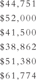
Calculate the mean, the median, and the mode.
Add another salary, $97,582. Calculate the mean, median, and mode again. How does this new salary affect the calculations?
Calculate the range, variance, and standard deviation for the original salary data.
How does the range change when you include the outlier salary, $97,582?
Question 4.19
The Mount Washington Observatory (MWO) in New Hampshire claims to have the world’s worst weather. Below are some data on the weather extremes recorded at the MWO.
| Month | Normal Daily Maximum (°F) | Normal Daily Minimum (°F) | Record Low in °F (Year) | Peak Wind Gust in Miles per Hour (Year) |
|---|---|---|---|---|
| January | 14.0 | −3.7 | −47 (1934) | 173 (1985) |
| February | 14.8 | −1.7 | −46 (1943) | 166 (1972) |
| March | 21.3 | 5.9 | −38 (1950) | 180 (1942) |
| April | 29.4 | 16.4 | −20 (1995) | 231 (1934) |
| May | 41.6 | 29.5 | −2 (1966) | 164 (1945) |
| June | 50.3 | 38.5 | 8 (1945) | 136 (1949) |
| July | 54.1 | 43.3 | 24 (2001) | 154 (1996) |
| August | 53.0 | 42.1 | 20 (1986) | 142 (1954) |
| September | 46.1 | 34.6 | 9 (1992) | 174 (1979) |
| October | 36.4 | 24.0 | −5 (1939) | 161 (1943) |
| November | 27.6 | 13.6 | −20 (1958) | 163 (1983) |
| December | 18.5 | 1.7 | −46 (1933) | 178 (1980) |
Calculate the mean and median normal daily minimum temperature across the year.
Calculate the mean, median, and mode for the record low temperatures.
Calculate the mean, median, and mode for the peak wind-
gust data. When no mode appears in the raw data, we can compute a mode by breaking the data into intervals. How might you do this for the peak wind-
gust data? Calculate the range, variance, and standard deviation for the normal daily minimum temperature across the year.
Calculate the range, variance, and standard deviation for the record low temperatures.
Calculate the range, variance, and standard deviation for the peak wind-
gust data.
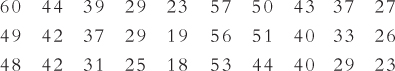
Question 4.20
Calculate the range and the interquartile range for the following set of data. Explain why they are so different.
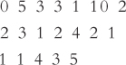
Question 4.21
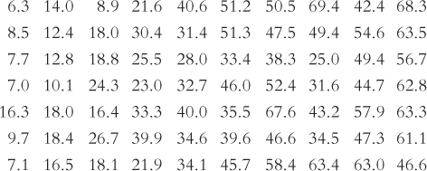
Calculate the interquartile range for the following set of data:

Question 4.22
Using the data presented in Exercise 4.19, calculate the interquartile range for peak wind gust.
Question 4.23
Why is the interquartile range you calculated for Exercise 4.22 so much smaller than the range you calculated in Exercise 4.19?
Question 4.24
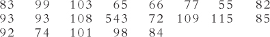
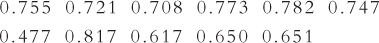
Here are the 2012 U.S. News & World Report data on acceptance rates at the top 70 national universities. These are the percentages of accepted students out of all students who applied.
Calculate the mean of these data, showing that you know how to use the symbols and formula.
Determine the median of these data.
Describe the variability in these data by computing the range.
Describe the variability in these data by computing the interquartile range.
Applying the Concepts
Question 4.25
Mean versus median for salary data: In Exercises 4.17 and 4.18, we saw how the mean and median changed when an outlier was included in the computations. If you were reporting the “average” salary at a company, how might the mean and median give different impressions to potential applicants?
Question 4.26
Mean versus median for temperature data: For the data in Exercise 4.19, the “normal” daily maximum and minimum temperatures recorded at the Mount Washington Observatory are presented for each month. These are likely to be measures of central tendency for each month over time. Explain why these “normal” temperatures might be calculated as means or medians. What would be the reasoning for using one type of statistic over the other?
97
Question 4.27
Mean versus median for depression scores: A depression research unit recently assessed seven participants chosen at random from the university population. Is the mean or the median a better indicator of the central tendency of these seven participants? Explain your answer.
Question 4.28
Measures of central tendency for weather data: The “normal” weather data from the Mount Washington Observatory are broken down by month. Why might you not want to average across all months in a year? How else could you summarize the year?
Question 4.29
Outliers, central tendency, and data on wind gusts: There appears to be an outlier in the data for peak wind gust recorded on top of Mount Washington (see the data in Exercise 4.19). Where do you see an outlier and how does excluding this data point affect the different calculations of central tendency?
Question 4.30
Measures of central tendency for measures of baseball performance: Here are winning percentages for 11 baseball players for their best 4-
What is the mean of these scores?
What is the median of these scores?
Compare the mean and the median. Does the difference between them suggest that the data are skewed very much?
Question 4.31
Mean versus median in “real life”: Briefly describe a real-
Question 4.32
Descriptive statistics in the media: Find an advertisement for an anti-
What does the ad promise that this product will do for the consumer?
What data does it offer for its promised benefits? Does it offer any descriptive statistics or merely testimonials? If it offers descriptive statistics, what are the limitations of what they report?
If you were considering this product, what measures of central tendency would you most like to see? Explain your answer, noting why not all measures of central tendency would be helpful.
If a friend with no statistical background were considering this product, what would you tell him or her?
Question 4.33
Descriptive statistics in the media: When there is an ad on TV for a body-
What kind of data is being presented in these ads?
What statistics could be presented to help inform the public about how much “individual results might vary”?
Question 4.34
Range of data for Canadian TV ratings: BBM Canada collects television ratings data (http:/
What is the range of these data?
What is the interquartile range of these data?
How does the IQR you calculated in part (b) differ from the range you calculated in part (a), and why is it different?
Question 4.35
Descriptive statistics for data from the National Survey of Student Engagement: The National Survey of Student Engagement (NSSE) asked U.S. students how many 20-
Calculate the mean of these data using the symbols and formula.
Calculate the variance of these data using the symbols and formula; also use columns to show all calculations.
Calculate the standard deviation using the symbols and formula.
In your own words, describe what the mean and standard deviation of these data tell us about these scores.
Question 4.36
Statistics versus parameters: For each of the following situations, state whether the mean would be a statistic or a parameter. Explain your answer.
According to 2011 Canadian census data, the median family income in British Columbia was $66,970, lower than the national average of $69,860.
In the 2010–
2011 soccer season, the stadiums of teams in the English Premier League had a mean capacity of 38,391 fans. The General Social Survey (GSS) includes a vocabulary test in which participants are asked to choose the appropriate synonym from a multiple-
choice list of five words (e.g., beast with the choices afraid, words, large, animal, and separate). The mean vocabulary test score was 5.98. The National Survey of Student Engagement (NSSE) asked students at participating institutions how often they discussed ideas or readings with professors outside of class. Among the 19 national universities that made their data public, the mean percentage of U.S. students who responded “Very often” was 8%.
Question 4.37
Central tendency and the shapes of distributions: Consider the many possible distributions of grades on a quiz in a statistics class; imagine that the grades could range from 0 to 100. For each of the following situations, give a hypothetical mean and median (that is, make up a mean and a median that might occur with a distribution that has this shape). Explain your answer.
Normal distribution
Positively skewed distribution
Negatively skewed distribution
Question 4.38
Shapes of distributions: For each of the following, state whether the distribution is more likely to be unimodal or bimodal. Explain your answer.
Age of patients in a hospital maternity ward
University students’ depression scores on a Beck Depression Inventory
GRE scores of applicants to sociology graduate programs
The cost of an AIDS drug that is sold in developed countries in Europe as well as in developing countries in Africa
Question 4.39
Outliers, Hurricane Sandy, and a rat infestation: In a New York Times article, reporter Cara Buckley described the influx of rats inland from the New York City shoreline following the flooding of Hurricane Sandy (2013). Buckley interviewed pest-
If you were to create a monthly average of rat violations over the course of the year before and after Hurricane Sandy, why would you not be able to make comparisons?
Explain how the removal of Zone A violations led both to the removal of an outlier and to inaccurate data.
Question 4.40
Outliers, H&M, and designer collaborations: The relatively low-
Question 4.41
Central tendency and outliers from growth-
Question 4.42
Measures of central tendency for percentages of advanced degrees: The U.S. Census Bureau collects and analyzes data on numerous aspects of American life by state, including the percentage of people with high school degrees, bachelor’s degrees, and advanced degrees. If you wanted to calculate the “average” percentage of people with advanced degrees across all states, would you report a mean, a median, or a mode? Explain your answer clearly.
Question 4.43
Mean versus median for age at first marriage: The mean age at first marriage was 31.1 for men and 29.1 for women in Canada in 2008 (http:/
Question 4.44
Range, world records, and a long chain of friendship bracelets: Guinness World Records reported that elementary school students in Pennsylvania created a chain of friendship bracelets that was a world record 2678 feet long as part of an anti-
99
Putting It All Together
Question 4.45
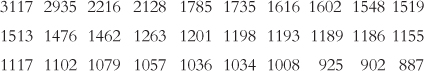
Descriptive statistics and basketball wins: Here are the numbers of wins for the 30 National Basketball Association teams in the 2012–
Create a grouped frequency table for these data.
Create a histogram based on the grouped frequency table.
Determine the mean, median, and mode of these data. Use symbols and the formula when showing your calculation of the mean.
Using software, calculate the range and standard deviation of these data.
Write a one-
to two- paragraph summary describing the distribution of these data. Mention center, variability, and shape. Be sure to discuss the number of modes (i.e., unimodal, bimodal, multimodal), any possible outliers, and the presence and direction of any skew. State one research question that might arise from this data set.
Question 4.46
Central tendency and outliers for data on traffic deaths: Below are estimated numbers of annual road traffic deaths for 12 countries based on 2010 data from the World Health Organization (http:/
| Country | Number of Deaths |
|---|---|
| United States | 35,490 |
| Australia | 1363 |
| Canada | 2296 |
| Denmark | 258 |
| Finland | 272 |
| Germany | 3830 |
| Italy | 4371 |
| Japan | 6625 |
| Malaysia | 7085 |
| Portugal | 1257 |
| Spain | 2478 |
| Turkey | 8758 |
Compute the mean and the median across these 12 data points.
Compute the range and interquartile range for these 12 data points.
Recalculate the statistics in part (a) and part (b) without the data point for the United States. How are these statistics affected by including or excluding the United States?
How might these numbers be affected by using traffic deaths per 100,000 people instead of using the number of traffic deaths overall?
Do you think that traffic deaths might vary by other personal or national characteristics? Could these represent confounds (as discussed in Chapter 1)?