7.3 An Example of the z Test
The story of the doctor tasting tea inspired statisticians to use hypothesis testing as a way to understand the many mysteries of human behavior. In this next section, we apply what we’ve learned about hypothesis testing—
174
EXAMPLE 7.5
Under Mayor Michael Bloomberg, New York City developed legislation targeted at public health issues, such as a 2003 ban on smoking in restaurants and bars. In 2008, New York became the first U.S. city to require that chain restaurants post calorie counts for all menu items.
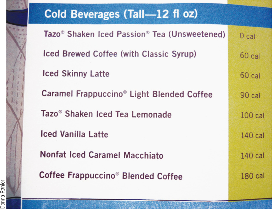
The research team of Bollinger, Leslie, and Sorensen (2010) wanted to test the law’s effectiveness, so for more than a year they gathered data on every transaction at Starbucks coffee shops in several U.S. cities. They determined a population mean of 247 calories in products purchased by customers at stores without calorie postings. Based on the range of 0 to 1208 calories in customer transactions, we estimate a standard deviation of approximately 201 calories, which we’ll use as the population standard deviation for this example.
The researchers also recorded calories for a sample in New York City after calories were posted on Starbucks menus. They reported a mean of 232 calories per purchase, a decrease of 6%. For the purposes of this example, we’ll assume a sample size of 1000. Here’s how to apply hypothesis testing when comparing a sample of customers at Starbucks with calories posted on their menus to the general population of customers at Starbucks without calories posted on their menus.
We’ll use the six steps of hypothesis testing to analyze the calorie data. These six steps will tell us if customers visiting a Starbucks with calories listed on the menu consume fewer calories, on average, than customers visiting a Starbucks without calories listed on the menu. In fact, we use the six-
STEP 1: Identify the populations, distribution, and assumptions.
First, we identify the populations, comparison distribution, and assumptions, which help us to determine the appropriate hypothesis test. The populations are (1) all customers at those Starbucks with calories posted on the menu (whether or not the customers are in the sample) and (2) all customers at those Starbucks without calories posted on the menu. Because we are studying a sample rather than an individual, the comparison distribution is a distribution of means. We compare the mean of the sample of 1000 people visiting those Starbucks that have calories posted on the menu (selected from the population of all people visiting those Starbucks with calories posted) to a distribution of all possible means of samples of 1000 people (selected from the population of all people visiting those Starbucks that don’t have calories posted on the menu). The hypothesis test will be a z test because we have only one sample and we know the mean and the standard deviation of the population from the published norms.
Now let’s examine the assumptions for a z test. (1) The data are on a scale measure, calories. (2) We do not know whether sample participants were selected randomly from among all people visiting those Starbucks with calories posted on the menu. If they were not, the ability to generalize beyond this sample to other Starbucks customers would be limited. (3) The comparison distribution should be normal. The individual data points are likely to be positively skewed because the minimum score of 0 is much closer to the mean of 247 than it is to the maximum score of 1208. However, we have a sample size of 1000, which is greater than 30; so based on the central limit theorem, we know that the comparison distribution—
175
Summary: Population 1: All customers at those Starbucks that have calories posted on the menu. Population 2: All customers at those Starbucks that don’t have calories posted on the menu.
The comparison distribution will be a distribution of means. The hypothesis test will be a z test because we have only one sample and we know the population mean and standard deviation. This study meets two of the three assumptions and may meet the third. The dependent variable is scale. In addition, there are more than 30 participants in the sample, indicating that the comparison distribution will be normal. We do not know whether the sample was randomly selected, however, so we must be cautious when generalizing.
STEP 2: State the null and research hypotheses.
Next we state the null and research hypotheses in words and in symbols. Remember, hypotheses are always about populations, not samples. In most forms of hypothesis testing, there are two possible sets of hypotheses: directional (predicting either an increase or a decrease, but not both) or nondirectional (predicting a difference in either direction).
The first possible set of hypotheses is directional. The null hypothesis is that customers at those Starbucks that have calories posted on the menu do not consume fewer mean calories than customers at those Starbucks that don’t have calories posted on the menu; in other words, they could consume the same or more mean calories, but not fewer. The research hypothesis is that customers at those Starbucks that have calories posted on the menu consume fewer mean calories than do customers at Starbucks that don’t have calories posted on the menu. (Note that the direction of the hypotheses could be reversed.)
The symbol for the null hypothesis is H0. The symbol for the research hypothesis is H1. Throughout this text, we use μ for the mean because hypotheses are about populations and their parameters, not about samples and their statistics. So, in symbolic notation, the hypotheses are:

For the null hypothesis, the symbolic notation says that the mean calories consumed by those in population 1, customers at those Starbucks with calories posted on the menu, is not lower than the mean calories consumed by those in population 2, customers at those Starbucks without calories posted on the menu. For the research hypothesis, the symbolic notation says that the mean calories consumed by those in population 1 is lower than the mean calories consumed by those in population 2.
A one-
This hypothesis test is considered a one-
176
The second set of hypotheses is nondirectional. The null hypothesis states that customers at Starbucks with posted calories (whether in the sample or not) consume the same number of calories, on average, as customers at Starbucks without posted calories. The research hypothesis is that customers at Starbucks with posted calories (whether in the sample or not) consume a different average number of calories than do customers at Starbucks without posted calories. The means of the two populations are posited to be different, but neither mean is predicted to be lower or higher.
The hypotheses in symbols would be:

For the null hypothesis, the symbolic notation says that the mean number of calories consumed by those in population 1 is the same as the mean number of calories consumed by those in population 2. For the research hypothesis, the symbolic notation says that the mean number of calories consumed by those in population 1 is different from the mean number of calories consumed by those in population 2.
A two-
This hypothesis test is considered a two-
MASTERING THE CONCEPT
7.3: We conduct a one-
Summary: Null hypothesis: Customers at those Starbucks that have calories posted on the menu consume the same number of calories, on average, as do customers at Starbucks that don’t have calories posted on the menu—
STEP 3: Determine the characteristics of the comparison distribution.
Now we determine the characteristics that describe the distribution with which we will compare the sample. For z tests, we must know the mean and the standard error of the population of scores; the standard error for samples of this size is calculated from the standard deviation of the population of scores. Here, the population mean for the number of calories consumed by the general population of Starbucks customers is 247, and the standard deviation is 201. The sample size is 1000. Because we usually use a sample mean in hypothesis testing, rather than a single score, we must use the standard error of the mean instead of the population standard deviation (of the scores). The characteristics of the comparison distribution are determined as follows:
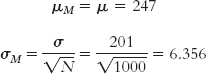
Summary: μM = 247; σM = 6.356.
177
STEP 4: Determine the critical values, or cutoffs.
Next we determine the critical values, or cutoffs, to which we can compare the test statistic. As stated previously, the research convention is to set the cutoffs to a p level of 0.05. For a two-
We know that 50% of the curve falls above the mean, and we know that 2.5% falls above the relevant z statistic. By subtracting (50% − 2.5% = 47.5%), we determine that 47.5% of the curve falls between the mean and the relevant z statistic. When we look up this percentage on the z table, we find a z statistic of 1.96. So the critical values are −1.96 and 1.96 (Figure 7-10).
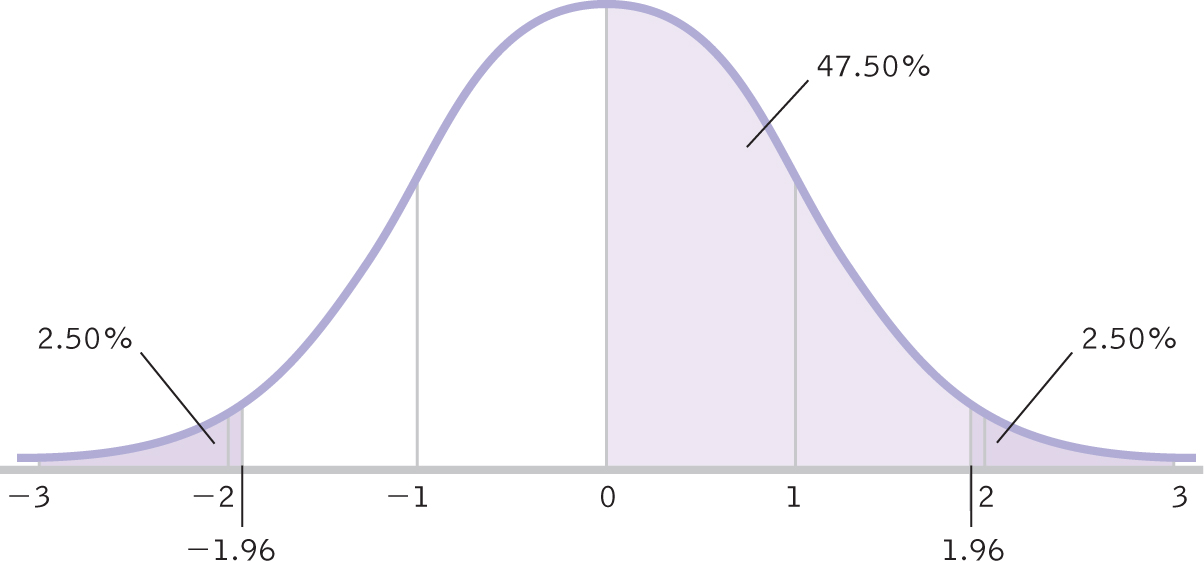
Figure 7-
Summary: The cutoff z statistics are −1.96 and 1.96.
STEP 5: Calculate the test statistic.
In step 5, we calculate the test statistic, in this case a z statistic, to find out what the data really say. We use the mean and standard error calculated in step 3:
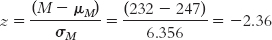
Summary: 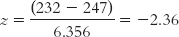
STEP 6: Make a decision.
Finally, we compare the test statistic to the critical values. We add the test statistic to the drawing of the curve that includes the critical z statistics (Figure 7-11). If the test statistic is in the critical region, we can reject the null hypothesis. In this example, the test statistic, −2.36, is in the critical region, so we reject the null hypothesis. An examination of the means tells us that the mean number of calories consumed by customers at those Starbucks with calories posted on the menu is lower than the mean number of calories consumed by customers at those Starbucks with no calories posted. So, even though we had nondirectional hypotheses, we can report the direction of the finding—
178
Figure 7-
If the test statistic is not beyond the cutoffs, we fail to reject the null hypothesis. This means that we can only conclude that there is no evidence from this study to support the research hypothesis. There might be a real mean difference that is not extreme enough to be picked up by the hypothesis test. We just can’t know.
Summary: We reject the null hypothesis. It appears that fewer calories are consumed, on average, by customers at Starbucks that post calories on the menus than by customers at Starbucks that do not post calories on the menu.
The researchers who conducted this study concluded that the posting of calories by restaurants does indeed seem to be beneficial. The 6% reduction may seem small, they admit, but they report that the reduction was larger—
Next Steps
Cleaning Data
In this section, we’ll consider three sources of what are sometimes called dirty data—missing data, misleading data, and outliers—
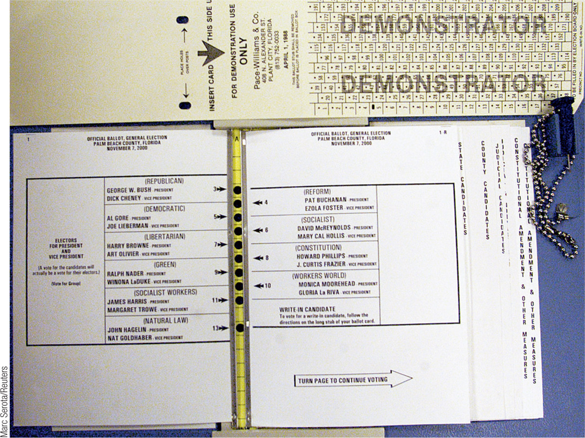
There are many causes of misleading data. For instance, maybe all participants didn’t understand a particular word. Even the cosmetic design of items on the page can be misleading. With the famous Florida “butterfly ballot” in the 2000 U.S. presidential election, a cosmetic flaw may have changed the outcome of a presidential election. This ballot was arranged like a book (instructions at the next of the page said to “TURN PAGE TO CONTINUE VOTING”). The customary style for reading a book in English is to read the entire left-
179
One type of misleading data is outliers. A single outlier can do significant damage to an otherwise cleanly collected and extremely useful data set. Outliers can be caused any number of ways—
Let’s consider some ways we can clean up dirty data. With missing data, the first question is, “Why is this data point missing?” If the reason is widespread, applies across most of the participants in a particular condition, or affects most of the data of some participants, then it might be wise to throw the data out. On the other hand, if we only have occasional loss of data, then we might be able to save the situation. What we need to know is how the researcher can best predict what participants would have answered. Here are three ways that researchers clean dirty data:
- Assign the mode or the mean for that variable, based on the other participants’ results.
- Assign the mode or the mean from the participant’s own responses if there are similar items in the database.
- Assign a random number that is within the range of possible numbers. (If you are using a 1–
7 scale, you wouldn’t assign the number 8.)
Misleading data present a slightly different problem, but one with similar solutions. For example, if we believe that a participant didn’t take the study seriously because he left much earlier than anyone else and drew a large circle around all the number 7’s, then we should probably just ignore those data. But if the possibly misleading data are only occasional and appear to be mistakes, then we have to make a judgment call. We may decide to use one of the solutions that we discussed for addressing missing data.
180
Outliers also can be a type of misleading data. Some problems with outliers are easy to resolve. For example, let’s say 120 participants in a sample completed a version of the Stroop test within a range of 90 seconds to 155 seconds, but one participant completed it in 12 seconds. She might be a visual-
The most interesting thing about dirty data is how the researcher addresses the problem. Judgment calls need to be made, of course, but the best solution is to report everything so that other researchers can assess the trade-
CHECK YOUR LEARNING
Reviewing the Concepts
- We conduct a z test when we have one sample and we know both the mean and the standard deviation of the population.
- We must decide whether to use a one-
tailed test , in which the hypothesis is directional, or a two-tailed test , in which the hypothesis is nondirectional. - One-
tailed tests are rare in the research literature. - The problem of dirty data can show up in three ways: missing data, misleading data, and outliers. A variety of techniques can be used to address dirty data, and researchers should report whatever techniques they chose to use when reporting their data.
Clarifying the Concepts
- 7-
11 What does it mean to say a test is directional or nondirectional?
Calculating the Statistics
- 7-
12 Calculate the characteristics (μM and σM) of a comparison distribution for a sample mean based on 53 participants when the population has a mean of 1090 and a standard deviation of 87. - 7-
13 Calculate the z statistic for a sample mean of 1094 based on the sample of 53 people when μ = 1090 and σ = 87.
Applying the Concepts
- 7-
14 According to the Web site for the Coffee Research Institute (http://www.coffeeresearch.org/ ), the average coffee drinker in the United States consumes 3.1 cups of coffee daily. Let’s assume the population standard deviation is 0.9 cup. Jillian decides to study coffee consumption at her local coffee shop. She wants to know if people sitting and working in a coffee shop drink a different amount of coffee from what might be expected in the general U.S. population. Throughout the course of 2 weeks, she collects data on 34 people who spend most of the day at the coffee shop. The average number of cups consumed by this sample is 3.17 cups. Use the six steps of hypothesis testing to determine whether Jillian’s sample is statistically significantly different from the population mean.market/ usa.htm
Solutions to these Check Your Learning questions can be found in Appendix D.
181