9.1 The t Distributions
The t distributions (note the plural) help us specify how confident we can be about research findings. We want to know whether we can generalize what we have learned about one sample to a larger population. The t test, based on the t distributions, tells us how confident we can be that the sample differs from the larger population.
The t distributions are more versatile than the z distribution because we can use them when (a) we don’t know the population standard deviation as we’ll learn in this chapter, and (b) we are comparing two samples as we’ll learn in chapters 10 and 11. Figure 9-1 demonstrates that there are many t distributions—
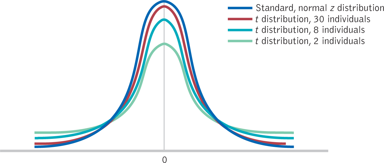
Figure 9-
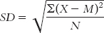
Estimating Population Standard Deviation from a Sample
Before we conduct a single-
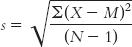
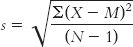
We need to make a correction to this formula to account for the fact that there is likely to be some level of error when we estimate the population standard deviation from a sample. Specifically, any given sample is likely to have somewhat less spread than does the entire population. One tiny alteration of this formula leads to a slightly larger and more accurate standard deviation. Instead of dividing by N, we divide by (N − 1) to get the mean of the squared deviations. Subtraction is the key. For example, if the numerator were 90 and the denominator (N) were 10, the answer would be 9; if we divide by (N − 1) = (10 − 1) = 9, the answer would be 10, a slightly larger value. So the formula is:
MASTERING THE FORMULA
9-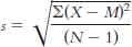 . We subtract 1 from the sample size in the denominator to correct for the probability that the sample standard deviation slightly underestimates the actual standard deviation in the population.
224

Notice that we call this standard deviation s instead of SD. We still use Latin rather than Greek letters because it is a statistic (from a sample) rather than a parameter (from a population). From now on, we will calculate the standard deviation in this way because we will be estimating the population standard deviation.
Let’s apply the new formula for standard deviation to a situation that involves a familiar activity: multitasking. Employees were observed at one of two high-
Suppose you were a manager at one of these firms and decided to reserve a period from 1:00 to 3:00 each afternoon during which employees could not interrupt one another, but might still be interrupted by people outside the company. To test the intervention, you observe five employees and develop a score for each—
EXAMPLE 9.1
To calculate the estimated standard deviation for the population, there are two steps.
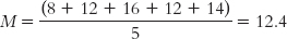
STEP 1: Calculate the sample mean.
Even though we know the population mean (11), we use the sample mean to calculate the corrected sample standard deviation. The mean for these scores is:
STEP 2: Use the sample mean in the corrected formula for the standard deviation.
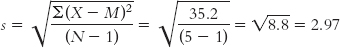
Remember, the easiest way to calculate the numerator under the square root sign is by first organizing the data into columns, as shown here:
| X | X − M | (X − M)2 |
|---|---|---|
| 8 | −4.4 | 19.36 |
| 12 | −0.4 | 0.16 |
| 16 | 3.6 | 12.96 |
| 12 | −0.4 | 0.16 |
| 14 | 1.6 | 2.56 |
225

© Oliver Weiken/epa/Corbis
Thus, the numerator is:
Σ(X − M)2 = Σ(19.36 + 0.16 + 12.96 + 0.16 + 2.56) = 35.2
And given a sample size of 5, the corrected standard deviation is:
Calculating Standard Error for the t Statistic
MASTERING THE FORMULA
9- . It only differs from the formula for standard error we learned previously in that we use s instead of σ because we’re working from a sample instead of a population.
We now have an estimate of the standard deviation of the distribution of scores, but not an estimate of the spread of a distribution of means, the standard error. As we did with the z distribution, we make the spread smaller to reflect the fact that a distribution of means is less variable than a distribution of scores. We do this in exactly the same way that we adjusted for the z distribution. We divide s by  . The formula for the standard error as estimated from a sample, therefore, is:

Notice that we have replaced σ with s because we are using the corrected sample standard deviation rather than the population standard deviation.
EXAMPLE 9.2
Here’s how we convert the corrected standard deviation of 2.97 to a standard error. The sample size was 5, so we divide by the square root of 5:
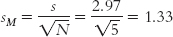
So the standard error is 1.33. Just as the central limit theorem predicts, the standard error for the distribution of sample means is smaller than the standard deviation of sample scores. (Note: This step can lead to a common mistake. Because we implemented a correction when calculating s, students often want to implement an extra correction here by dividing by  . Do not do this! We still divide by
in this step. There is no need for a further correction to the standard error.)
. Do not do this! We still divide by
in this step. There is no need for a further correction to the standard error.)
226
Using Standard Error to Calculate the t Statistic
The t statistic indicates the distance of a sample mean from a population mean in terms of the estimated standard error.
We now have the tools necessary to conduct the single-
MASTERING THE FORMULA
9- . It only differs from the formula for the z statistic in that we use sM instead of σM because we use the sample to estimate standard error rather than using the actual population standard error.
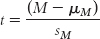
Note that the denominator is the only difference between this formula for the t statistic and the formula used to compute the z statistic for a sample mean. The corrected denominator makes the t statistic smaller and thereby reduces the probability of having an extreme t statistic. That is, a t statistic is not as extreme as a z statistic; in scientific terms, it’s more conservative.
EXAMPLE 9.3
The t statistic for the sample of five scores representing minutes until interruptions is:
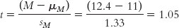
As part of the six steps of hypothesis testing, the t statistic can help us make an inference about whether the ban on internal interruptions affected the average number of minutes until an interruption.
CHECK YOUR LEARNING
Reviewing the Concepts
- We use t distributions when we do not know the population standard deviation and are comparing only two groups.
- The two groups may be a sample and a population, or two samples as part of a within-
groups design or a between- groups design. - The formula for the t statistic for a single-
sample t test is the same as the formula for the z statistic for a distribution of means, except that we use estimated standard error in the denominator rather than the actual standard error for the population. - We calculate estimated standard error by dividing by N − 1, rather than dividing by N, when calculating standard error.
Clarifying the Concepts
- 9-
1 What is the t statistic?
Calculating the Statistics
- 9-
2 Calculate the standard deviation for a sample (SD) and as an estimate of the population (s) using the following data: 6, 3, 7, 6, 4, 5. - 9-
3 Calculate standard error for t for the data given in Check Your Learning 9-2.
227
Applying the Statistics
- 9-
4 In the discussion of a study on multitasking (Mark et al., 2005), we imagined a follow-up study in which we measured time until a task was interrupted. For each of the five employees, let’s now examine time until work on the initial task was resumed at 20, 19, 27, 24, and 18 minutes. Remember that the original research showed it took 25 minutes on average for an employee to return to a task after being interrupted. - What distribution would be used in this situation? Explain your answer.
- Determine the appropriate mean and standard deviation (or standard error) for this distribution. Show all your work; use symbolic notation and formulas where appropriate.
- Calculate the t statistic.
Solutions to these Check Your Learning questions can be found in Appendix D.