Question 9.1

Question 9.2

Question 9.3

Question 9.4

239

Question 9.5

Question 9.6

Question 9.7

Question 9.8

Question 9.9

Question 9.10

Question 9.11

Question 9.12

We use formulas to describe calculations. Find the error in each of the following formulas. Explain why each is incorrect and provide a correction.

Question 9.13

For the data 93, 97, 91, 88, 103, 94, 97, calculate the standard deviation under both of these conditions:

1. For this sample

2. As an estimate of the population

3. Calculate the standard error for t using symbolic notation.

4. Calculate the t statistic, assuming μ = 96.

Question 9.14

For the data 1.01, 0.99, 1.12, 1.27, 0.82, 1.04, calculate the standard deviation under both of the following conditions. (Note: You will have to carry some calculations out to the third decimal place to see the difference in calculations.)

1. For the sample

2. As an estimate of the population

3. Calculate the standard error for t using symbolic notation.

4. Calculate the t statistic, assuming μ = 0.96.

Question 9.15

Identify the critical t value in each of the following circumstances:

1. One-tailed test, df = 73, p level of 0.10

2. Two-tailed test, df = 108, p level of 0.05

3. One-tailed test, df = 38, p level of 0.01

Question 9.16

Calculate degrees of freedom and identify the critical t value for a single-sample t test in each of the following circumstances:

1. Two-tailed test, N = 8, p level of 0.10

2. One-tailed test, N = 42, p level of 0.05

3. Two-tailed test, N = 89, p level of 0.01

Question 9.17

Identify the critical t values for each of the following tests:

1. A single-sample t test examining scores for 26 participants to see if there is any difference compared to the population, using a p level of 0.05

2. A one-tailed, single-sample t test performed on scores on the Marital Satisfaction Inventory for 18 people who went through marriage counseling, as compared to the population of people who had not been through marital counseling, using a p level of 0.01

3. A two-tailed, single-sample t test, using a p level of 0.05, with 34 degrees of freedom

Question 9.18

Assume we know the following for a two-tailed, single-sample t test, at a p level of 0.05: μ = 44.3, N = 114, M = 43, s = 5.9.

1. Calculate the t statistic.

2. Calculate a 95% confidence interval.

3. Calculate the effect size using Cohen’s d.

Question 9.19

Assume we know the following for a two-tailed, single-sample t test: μ = 7, N = 41, M = 8.5, s = 2.1.

1. Calculate the t statistic.

2. Calculate a 99% confidence interval.

3. Calculate the effect size using Cohen’s d.

Question 9.20

Students in a statistics course reported the number of hours of sleep they get on a typical weeknight. These data appear below.

1. Create a dot plot of these data.

2. Use the dot plot to describe the distribution of the set of scores.

Question 9.21

The relation between the z distribution and the t distributions: For each of the problems described below, which are the same as some of those described in Exercise 9.17, identify what the critical z value would have been if there had been just one sample and we knew the mean and standard deviation of the population:

1. A single-sample t test examining scores for 26 participants to see if there is any difference compared to the population, using a p level of 0.05

2. A one-tailed, single-sample t test performed on scores on the Marital Satisfaction Inventory for 18 people who went through marriage counseling, using a p level of 0.01

3. A two-tailed, single-sample t test, using a p level of 0.05, with 34 degrees of freedom

4. Comparing the critical t values with the critical z values, explain how and why these are different.

240

Question 9.22

t statistics and standardized tests: On its Web site, the Princeton Review claims that students who have taken its course improve their Graduate Record Examination (GRE) scores, on average, by 210 points. (No other information is provided about this statistic.) Treating this average gain as a population mean, a researcher wonders whether the far cheaper technique of practicing for the GRE on one’s own would lead to a different average gain. She randomly selects five students from the pool of students at her university who plan to take the GRE. The students take a practice test before and after 2 months of self-study. They reported (fictional) gains of 160, 240, 340, 70, and 250 points. (Note that many experts suggest that the results from self-study are similar to those from a structured course for students who have the self-discipline to study on their own. Regardless of the format, preparation has been convincingly demonstrated to lead to increased scores, on average.)

1. Using symbolic notation and formulas (where appropriate), determine the appropriate mean and standard error for the distribution to which we will compare this sample. Show all steps of your calculations.

2. Using symbolic notation and the formula, calculate the t statistic for this sample.

3. As an interested consumer, what critical questions would you want to ask about the statistic reported by the Princeton Review? List at least three questions.

Question 9.23

Single-sample t test, military training, and anger: Bardwell, Ensign, and Mills (2005) assessed the moods of 60 male U.S. Marines following a month-long training exercise conducted in cold temperatures and at high altitudes. Negative moods, including fatigue and anger, increased substantially during the training and lasted up to 3 months after the training ended. Mean mood scores were compared to population norms for three groups: college men, adult men, and male psychiatric outpatients. Let’s examine anger scores for six Marines at the end of training; these scores are fictional, but their mean and standard deviation are very close to the actual descriptive statistics for the sample: 14, 12, 13, 12, 14, 15.

1. The population mean anger score for college men is 8.90. Conduct all six steps of a single-sample t test. Report the statistics as you would in a journal article.

2. Now calculate the test statistic to compare this sample mean to the population mean anger score for adult men (M = 9.20). You do not have to repeat all the steps from part (a), but conduct step 6 of hypothesis testing and report the statistics as you would in a journal article.

3. Now calculate the test statistic to compare this sample mean to the population mean anger score for male psychiatric outpatients (M = 13.5). Do not repeat all the steps from part (a), but conduct step 6 of hypothesis testing and report the statistics as you would in a journal article.

4. What can we conclude overall about Marines’ moods following high-altitude, cold-weather training?

Question 9.24

Consideration of Future Consequences and a dot plot: The following data are Consideration of Future Consequences (CFC) scores for 20, already arranged in order from lowest to highest:

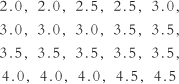
1. Construct a dot plot for these data.

2. What can you learn about the shape of this distribution from this plot?

Question 9.25

Credit card debt and dot plots: Below are the amounts of credit card debt reported by 27 men and 23 women.

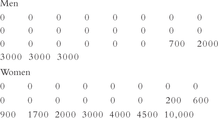
1. Construct stacked dot plots for these data.

2. What can we learn about these two distributions from this graph?

Question 9.26

Paid days off and the single-sample t test: The number of paid days off (e.g., vacation, sick leave) taken by eight employees at a small local business is compared to the national average. You are hired as a consultant by the new business owner to help her determine how many paid days off she should provide. In general, she wants to set some standard for her employees and for herself. Let’s assume your search on the Internet for data on paid days off leaves you with the impression that the national average is 15 days. The data for the eight local employees during the last fiscal year are: 10, 11, 8, 14, 13, 12, 12, and 27 days.

1. Write hypotheses for your research.

2. Which type of test would be appropriate to analyze these data in order to answer your question?

3. Before doing any computations, do you have any concerns about this research? Are there any questions you might like to ask about the data you have been given?

4. Calculate the appropriate t statistic. Show all of your work in detail.

5. Draw a statistical conclusion for this business owner.

6. Calculate the confidence interval.

7. Calculate and interpret the effect size.

8. Consider all the results you have calculated. How would you summarize the situation for this business owner? Identify the limitations of your analyses, and discuss the difficulties of making comparisons between populations and samples. Make reference to the assumptions of the statistical test in your answer.

9. After further investigation, you discover that one of the data points, 27 days, was actually the owner’s number of paid days off. Calculate the t statistic and draw a statistical conclusion, adapting for this new information by deleting that value. What changed in the re-analysis of the data?

10. Calculate and interpret the effect size, adapting for this new information by deleting the outlier of 27 days. What changed in the re-analyses of the data?

Question 9.27

Death row and the single-sample t test: The Florida Department of Corrections publishes an online death row fact sheet. It reports the average time on death row prior to execution as 11.72 years but provides no standard deviation. This mean is a parameter because it is calculated from the entire population of executed prisoners in Florida. Has the time spent on death row changed in recent years? According to the execution list linked to the same Web site, the six prisoners executed in Florida during the years 2003, 2004, and 2005 spent 25.62, 13.09, 8.74, 17.63, 2.80, and 4.42 years on death row, respectively. (All were men, although Aileen Wuornos, the serial killer portrayed by Charlize Theron in the 2003 film Monster, was among the three prisoners executed by the state of Florida in 2002; Wuornos spent 10.69 years on death row.)

1. Using symbolic notation and formulas (where appropriate), determine the appropriate mean and standard error for the distribution of means. Show all steps of your calculations.

2. Using symbolic notation and the formula, calculate the t statistic for time spent on death row for the sample of recently executed prisoners.

3. The execution list provides data on all prisoners executed since the death penalty was reinstated in Florida in 1976. Included for each prisoner are the name, race, gender, date of birth, date of offense, date sentenced, date arrived on death row, data of execution, number of warrants, and years on death row. State at least one hypothesis, other than year of execution, which could be examined using a t distribution and the comparison mean of 11.72 years on death row. Be specific about your hypothesis (and if you are interested, you can search for the data online).

4. What additional information would you need to calculate a z score for the length of time Aileen Wuornos spent on death row?

5. Write hypotheses to address the question “Has the time spent on death row changed in recent years?”

6. f. Using these data as “recent years” and the mean of 11.72 years as the comparison, answer the question based on the t statistic calculated in part (b), using alpha of 0.05.

7. Calculate the confidence interval for this statistic based on the data presented.

8. What conclusion would you make about your hypotheses based on this confidence interval? What can you say about the size of this confidence interval?

9. Calculate the effect size using Cohen’s d.

10. Evaluate the size of this effect.