Jeffrey Mitton and his colleagues found three genotypes (R²R², R²R³, and R³R³) at a locus encoding the enzyme peroxidase in ponderosa pine trees growing at Glacier Lake, Colorado. The observed numbers of these genotypes were

Are the ponderosa pine trees at Glacier Lake in Hardy–Weinberg equilibrium at the peroxidase locus?

Solution Strategy

What information is required in your answer to the problem?

The results of a chi-square test to determine whether the population is in Hardy-Weinberg equilibrium.

What information is provided to solve the problem?

Solution Steps

If the frequency of the R² allele equals p and the frequency of the R³ allele equals q, the frequency of the R² allele is

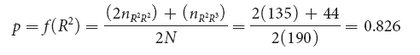
The frequency of the R³ allele is obtained by subtraction:

q = f(R³) = 1 – p = 0.174

The frequencies of the genotypes expected under Hardy–Weinberg equilibrium are then calculated by using p², 2pq, and q²:

R²R² = p² = (0.826)² = 0.683

R²R³ = 2pq = 2(0.826)(0.174) = 0.287

R³R³ = q² = (0.174)² = 0.03

Multiplying each of these expected genotypic frequencies by the total number of observed genotypes in the sample (190), we obtain the numbers expected for each genotype:

R²R² = 0.683 × 190 = 129.8

R²R³ = 0.287 × 190 = 54.5

R³R³ = 0.03 × 190 = 5.7

By comparing these expected numbers with the observed numbers of each genotype, we see that there are more R²R² and R³R³ homozygotes and fewer R²R³ heterozygotes in the population than we expect at equilibrium.

A chi-square goodness-of-fit test is used to determine whether the differences between the observed and the expected numbers of each genotype are due to chance:

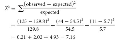
The calculated chi-square value is 7.16. To obtain the probability associated with this chi-square value, we determine the appropriate degrees of freedom.

So far, the chi-square test for assessing Hardy–Weinberg equilibrium has been identical with the chi-square tests that we used in Chapter 3 to assess progeny ratios in a genetic cross, where the degrees of freedom were n – 1 and n equaled the number of expected genotypes. For the Hardy–Weinberg test, however, we must subtract an additional degree of freedom because the expected numbers are based on the observed allelic frequencies; therefore, the expected numbers are not completely free to vary. In general, the degrees of freedom for a chi-square test of Hardy–Weinberg equilibrium equal the number of expected genotypic classes minus the number of associated alleles. For this particular Hardy–Weinberg test, the degree of freedom is 3 − 2 = 1.

After we have calculated both the chi-square value and the degrees of freedom, the probability associated with this value can be sought in a chi-square table (see Table 3.4). With 1 degree of freedom, a chi-square value of 7.16 has a probability between 0.01 and 0.001. Thus, the observed values differ significantly from the expected values, and the peroxidase genotypes observed at Glacier Lake are not likely to be in Hardy–Weinberg proportions.

The observed number of genotypes in a population can be compared with the expected Hardy–Weinberg proportions by using a chi-square goodness-of-fit test.