Concept 42.1: Populations Are Patchy in Space and Dynamic over Time

In Chapter 41 we saw that individual organisms are the fundamental units of all larger ecological systems. Many important insights are gained by focusing on these fundamental units, but additional insights arise by studying populations—groups of individuals of the same species. Populations have properties that individuals do not have, and we cannot understand larger ecological systems, such as communities, without understanding their component populations. One important property of populations is abundance because, together with the average properties of individuals, abundance determines a species’ ecological role in the larger community or ecosystem.

Humans have long had a practical interest in understanding what determines abundance because we want to manage our ecological interactions with other species. We want to know how to increase the abundance of organisms that provide us with resources such as food or fiber for clothing, how to conserve wild organisms that benefit us by acting as agents of pollination or pest control, and how to decrease the abundance of undesirable organisms such as crop pests, weeds, and pathogens. Understanding population ecology is a key to achieving these goals.

Population density and population size are two measures of abundance

“Abundance” has several meanings in ecology. We might consider a species abundant because there are many individuals in an area. If that same species occurs only in a small geographic region, however, we might consider it rare because the total number of individuals of that species is small. Depending on why they want to measure abundance, ecologists use one of two approaches. If they are interested in the causes or consequences of local abundance, they usually measure population density: the number of individuals per unit of area (for surface-dwelling organisms) or volume (for organisms that live in air, soil, or water). Alternatively, if ecologists are interested in the population as a whole, they usually measure population size: the number of individuals in the population.

Counting all the individuals in a population is practical only for very small populations in which individuals can be distinguished. For this reason, ecologists usually measure population density first. Then they multiply population density by the area or volume occupied by the entire population to estimate population size.

Abundance varies in space and over time

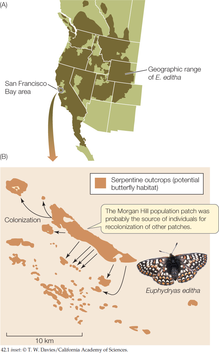
The abundance of organisms varies on several spatial scales. At the largest scale, as we saw in Chapter 41, many species are found only in a particular region, and their densities are zero elsewhere. Within that region, which is called the species’ geographic range, the species may be restricted to particular kinds of environments, often called habitats, which may themselves be patchily distributed. For example, Edith’s checkerspot butterfly (Euphydryas editha) is found from southern British Columbia and Alberta to Baja California, Nevada, Utah, and Colorado (FIGURE 42.1A). Within this geographic range, it occurs in the open habitats (coastal chaparral, meadows, grasslands, or open woodlands) where the plants that its caterpillars eat are found. In the San Francisco Bay area, suitable food plants grow only in soils derived from a chemically unique rock called serpentine (FIGURE 42.1B). Outcrops of serpentine rocks constitute habitat “islands” for the butterflies—that is, patches of suitable habitat separated by areas of unsuitable habitat. Habitat patchiness has consequences for abundance that we will explore in Concept 42.5.

Figure 42.1: Species Are Patchily Distributed on Several Spatial Scales (A) The geographic range of Edith’s checkerspot butterfly (Euphydryas editha) extends from British Columbia and Alberta to Baja California. (B) Within the geographic range, the butterflies occur in patches of suitable habitat which, in the San Francisco Bay area, are on serpentine soils. Arrows indicate colonization events that are discussed in Concept 42.5.

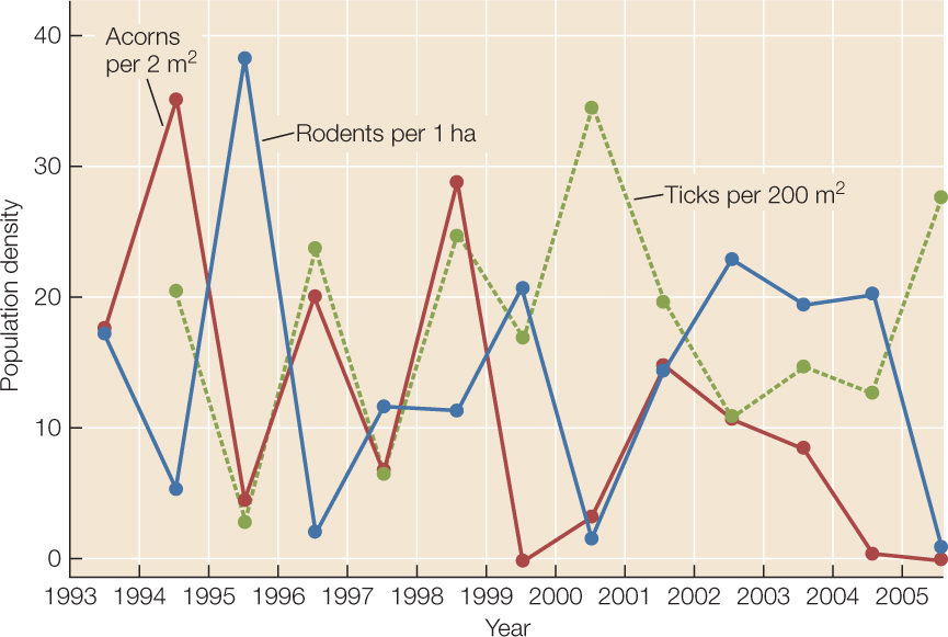
In any given locality, population densities are dynamic—they change over time. For example, abundances of rodents, blacklegged ticks, and oak acorns vary greatly from year to year in the forests described in the opening story (FIGURE 42.2).

Figure 42.2: Population Densities Are Dynamic Densities of acorns, rodents, and nymphal black-legged ticks varied over time in an oak forest near Millbrook, New York. (Notice that the population density of each organism is measured on a spatial scale appropriate for that organism’s average density; see Appendix C for definitions of units of area.)

Why do species abundances vary in time and space? To answer this question, we need to understand the processes that add individuals to or subtract them from populations.