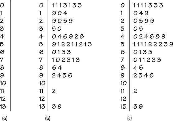
EXAMPLE 1.16 A Stemplot of T-Bill Interest Rates
tbill50
CASE 1.1 The histogram that we produced in Example 1.12 to examine the T-bill interest rates used all 2895 cases in the data set. To illustrate the idea of a stemplot, we take a simple random sample of size 50 from this data set. We learn more about how to take such samples in Chapter 3. Here are the data:
| 7.1 | 5.9 | 3.5 | 5.1 | 6.0 | 5.2 | 1.9 | 7.0 | 2.9 | 9.2 |
| 5.2 | 7.2 | 9.4 | 5.1 | 0.1 | 6.1 | 8.6 | 3.0 | 0.1 | 2.0 |
| 4.0 | 6.3 | 13.3 | 9.3 | 13.9 | 0.1 | 4.4 | 0.3 | 4.6 | 5.1 |
| 4.9 | 7.3 | 6.3 | 5.2 | 1.0 | 7.1 | 2.5 | 7.3 | 11.2 | 9.6 |
| 5.1 | 0.1 | 0.3 | 5.3 | 4.2 | 0.3 | 4.8 | 2.9 | 1.4 | 8.4 |
The original data set gave the interest rates with two digits after the decimal point. To make the job of preparing our stemplot easier, we first rounded the values to one place following the decimal.
Figure 1.9 illustrates the key steps in constructing the stemplot for these data. How does the stemplot for this sample of size 50 compare with the histogram based on all 2894 interest rates that we examined in Figure 1.6 (page 13)?
