Example 12.11

EXAMPLE 12.11 Absenteeism Rate $p$ Chart

absent

CASE 12.3 Are your actions effective? You hope to see a reduction in absenteeism. To view progress (or lack of progress), you will keep a $p$ chart of the proportion of absentees. The plant has 987 production workers. For simplicity, you just record the number who are absent from work each day. Only unscheduled absences count, not planned time off such as vacations.

Each day you will plot

$\hat{p} = \frac{number of workers absent}{987}$

You first look back at data for the past three months. There were 64 workdays in these months. The total workdays available for the workers was

$(64) (987) = 63,168 person-days$

Page 633

Absences among all workers totaled 7580 person-days. The average daily proportion absent was therefore

$\begin{array}{l} \bar{p} & = & \frac{total days absent}{total days available for work} \\ = & \frac{7580}{63,168} = 0.120 \end{array}$

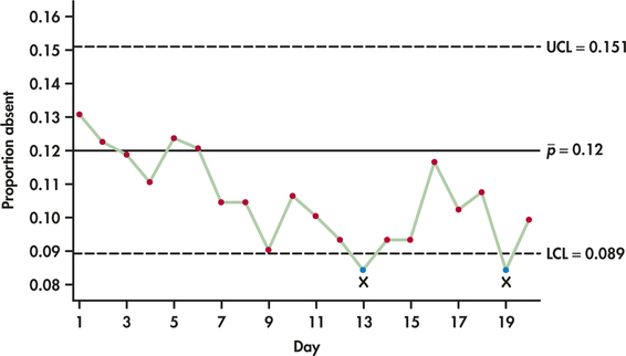
The daily rate has been in control at this level.

These past data allow you to set up a $p$ chart to monitor future proportions absent:

$\begin{array}{l} UCL & = & \bar{p} + 3 \sqrt{\frac{\bar{p} (1 - \bar{p})}{n}} = 0.120 + 3 \sqrt{\frac{(0.120) (0.880)}{987}} \\ = & 0.120 + 0.031 = 0.151 \\ CL & = & \bar{p} = 0.120 \\ LCL & = & \bar{p} - 3 \sqrt{\frac{\bar{p} (1 - \bar{p})}{n}} = 0.120 - 3 \sqrt{\frac{(0.120) (0.880)}{987}} \\ = & 0.120 - 0.031 = 0.089 \end{array}$

Table 12.8 gives the data for the next four weeks. Figure 12.18 is the $p$ chart.

Table 12.11: TABLE 12.8 Proportions of workers absent during four weeks

Day	M	T	W	Th	F	M	T	W	Th	F
Workers absent	129	121	117	109	122	119	103	103	89	105
Proportion $\hat{p}$	0.131	0.123	0.119	0.110	0.124	0.121	0.104	0.104	0.090	0.106
Workers absent	99	92	83	92	92	115	101	106	83	98
Proportion $\hat{p}$	0.100	0.093	0.084	0.093	0.093	0.117	0.102	0.107	0.084	0.099

FIGURE 12.18 Prospective-monitoring

$p$ chart for daily proportion of workers absent over a four-week period, Example 12.11. The lack of control shows an improvement (decrease) in absenteeism. Update the chart to continue monitoring the process.