EXAMPLE 13.12 Monthly Cable Sales

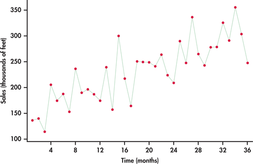
Consider the monthly sales data for festoon cable manufactured by a global distributor of electric wire and cable taken over a three-year horizon starting with January.¹⁰ Festoon cable is a flat cable used in overhead material-handling equipment such as cranes, hoists, and overhead automation systems. The sales data are specifically the total number of linear feet (in thousands of feet) sold in a given month. In the time plot of Figure 13.19, the upward trend is clearly visible.

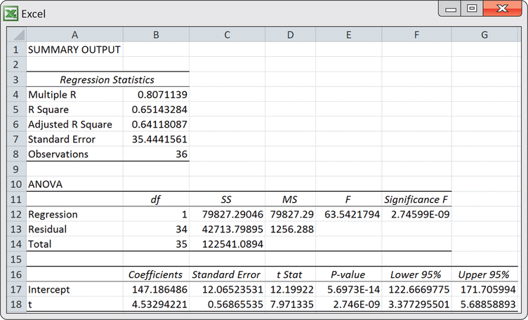
If we ignore the line connections made between successive observations, the plot of Figure 13.19 can be viewed as a scatterplot of the response variable (sales) against the explanatory variable, which is simply the indexed numbers 1, 2, …, 36. With this perspective we can use the ideas of simple linear regression (Chapter 2) and software to estimate the upward trend. From the following Excel regression output, we estimate the linear trend to be

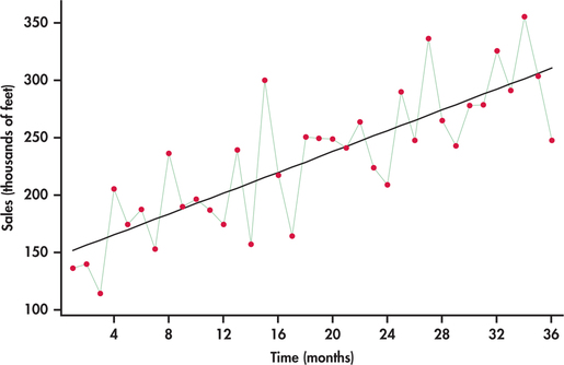
where is a time index of the number of months elapsed since the first month of the time series; that is, corresponds to first month (January), corresponds to second month (February), and so on. Figure 13.20 is the time plot of Figure 13.19 with the estimated trend line superimposed.

666

The equation of the line provides a mathematical model for the observed trend in sales. The estimated slope of 4.533 indicates that festoon cable sales increased an average of 4.533 thousand feet per month.