Example 13.16

EXAMPLE 13.16 Monthly warehouse Club and Superstore Sales

club

The seasonal pattern in the sales data seems to repeat every 12 months, so we begin by creating $12 - 1 = 11$ indicator variables.

$\begin{array}{l} J a n = {\begin{array}{l} 1 & if the month is January \\ 0 & otherwise \end{array} \\ F e b = {\begin{array}{l} 1 & if the month is February \\ 0 & otherwise \end{array} \\ ⋮ \\ N o v = {\begin{array}{l} 1 & if the month is November \\ 0 & otherwise \end{array} \end{array}$

December data are indicated when all 11 indicator variables are 0.

We can extend the trend model with these indicator variables. The new model captures the trend along with the seasonal pattern in the time series.

${SALES}_{t} = β_{0} + β_{1} t + β_{2} J a n + \dots + β_{12} N o v + ε_{t}$

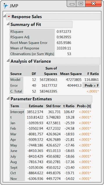
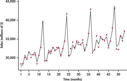
Fitting this multiple regression model to our data, we get the regression output shown in Figure 13.29. Figure 13.30 displays the time plot of sales observations with the trend-and-season model superimposed. You can see the dramatic improvement over the trend-only model by comparing Figure 13.28 with Figure 13.30. The improved model fit is reflected in the $R^{2}$ -values for the two models: $R_{2} = 97.2 %$ for the trend-and-season model and $R_{2} = 32.3 %$ for the trend-only model. The significance of seasonal

Page 673

FIGURE 13.29 JMP Trend-and-season regression output for monthly warehouse club and superstore sales.

FIGURE 13.30 Trend-and-season model fitted to monthly warehouse club and superstore sales.

Page 674

variables can be collectively tested with an $F$ -test introduced in Chapter 11. The heart of the test is based on the change in $R^{2}$ . In our case, we find the seasonal variables significantly contribute to the prediction of sales ( $F = 85.15$ and $P < 0.001$ ).

Reminder

$F$ test for collection of regression coefficients, p. 559

Notice from the regression output that all the monthly coefficients are negative. The reason for this is because of the exclusion of the December indicator variable in the model. December would be associated with all the other indicator variables being 0. When all of these 0’s are substituted into the model, we obtain a baseline trend model fit for the Decembers. Each of the other months have an estimated trend line a certain amount below December depending on the magnitude of the month’s coefficient.