EXAMPLE 13.18 Fitting and Forecasting Amazon Sales

CASE 13.1 In Case 13.1 (page 647), we observed that the time series was growing at an increasing rate, which leads us to consider an exponential trend model. Additionally, we saw that the seasonal variation increases with the growth of sales. This indicates that an additive seasonal model is probably not the best choice.

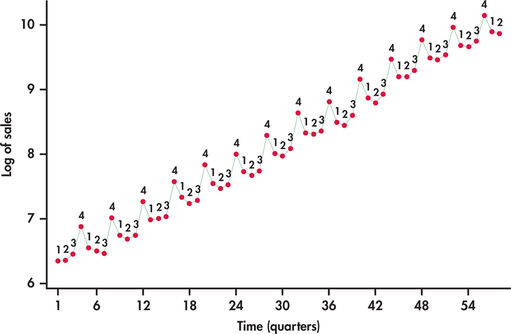
It seems that this data series is a good candidate for logarithmic transformation. Figure 13.31 displays the sales series in logged units. Compare this time plot with Figure 13.4 (page 648). In logged units, the trend is now nearly perfectly linear. Furthermore, the seasonal variation from the trend is much more constant. These facts together imply that we can model logged sales as a linear trend with additive seasonal indicator variables:

where Q1, Q2, and Q3 are indicator variables for quarters 1, 2, and 3, respectively. Statistical software calculates the fitted model to be

To make predictions of sales in the original units, millions of dollars, we can first predict sales in logged units using the preceding fitted equation. The series ended with the second quarter of 2014 and with . The next period would than be the third quarter of 2014 with , which means a forecast of

At this stage, we untransform the log prediction value by applying the exponential function, which on your calculator is the key.

676

However, it should be noted that by exponentiating the predicted value of log(), the untransformed value provides an estimate of the median response at the given values of the predictor variables. Recall that standard regression provides an estimate for the mean response at given values of the predictor variables. If prediction of the mean is desired, then an adjustment factor must be applied to the untranformed prediction.¹⁵

The adjustment is accomplished by multiplying the untransformed prediction by , where is the regression standard error from the log-based regression. From the regression output for the fitting of logged sales, we find . The predicted mean sales is then

In this application, the regression standard error is small, which results in only a slight adjustment to the initial untransformed value. The forecast is in millions of dollars. So third-quarter sales are forecasted to be about $21.332 billion.