EXAMPLE 13.25 Fitting and Forecasting Amazon Sales

CASE 13.1 Example 13.19 (page 678) showed us that the trend-and-season model given in Example 13.18 (pages 675–676) fails to capture the autocorrelation effect between successive observations. One strategy is to add a lag variable to the trend-and-seasonal model. In other words, we need to consider a model for logged sales that combines all the effects:

From software, we find the estimated model to be

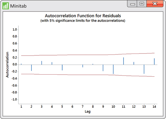
Figure 13.44 shows the ACF for the residuals from the above fit. Compare this ACF with the trend-and-seasonal residuals ACF of Figure 13.34 (page 678). We can see that the lag effects have been captured and thus result in a better fitting model. In terms of forecasting, the series ends with second-quarter 2014 sales of $19,340 (in millions). The ending quarter is the 58th period in the series, so our notation is $y_{58}=19,340$.

First, use the model to forecast the logarithm of third-quarter 2014 sales:

We can now untransform the log predicted value:

Recall from the discussion of Example 13.18 (pages 675–676) that the preceding fitted value provides a prediction of median sales. If we want a prediction of mean sales, we need to obtain the regression standard error from our log fit. From the regression output for the fitting of logged sales, we find $s=0.0410473$. The predicted mean sales is then