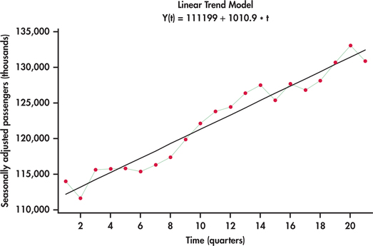
EXAMPLE 13.30 Seasonally Adjusted Light Rail Usage
rail
By again rearranging the trend-times-seasonal model, we obtain
ySEASON=TREND
This ratio tells us how to seasonally adjust a series. In particular, by dividing the original series by the seasonal component, we are then left with the trend component with no seasonality. Dividing each observation of the original series by its respective seasonal ratio found in Example 13.29 results in the series shown in Figure 13.50. This adjusted series does not show the regular ups and downs of the original unadjusted data. At this stage, we can come up with a trend line equation using regression as seen in Figure 13.50. Our trend-and-season predictive model is then
ˆyt=(111,199+1010.9t)×SR
where SR is the seasonality ratio for the appropriate quarter corresponding to the value of t.

To illustrate the computation of a forecast, we note that the series ended on the first quarter with t=21. This means that the next period in the future is the second quarter with t=22. Accordingly, the forecast would be
ˆyt=[111,199+1010.9(22)]×1.016=135,573.82