EXAMPLE 13.32 Disney Returns

In Example 13.1 (pages 645–646), we first studied the weekly returns of Disney stock with a time plot. The time plot along with the runs test (Example 13.5, page 653) and ACF (Example 13.6, pages 653–654) showed that the returns series is consistent with a random series.

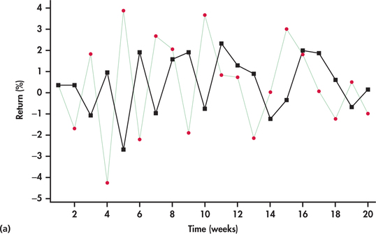
Figure 13.52(a) shows the last 20 observations of the series with forecasts based on . With a smoothing constant of 0.7, the one-step-ahead forecasts are close in value to the most recent observation in the returns series. Because the returns are bouncing around randomly, we find that the forecasts are also bouncing around randomly but are often considerably off from the actual observations they are attempting to predict. Looking closely at Figure 13.52(a), we see that when a return is higher than the average, then the forecast for the next period’s return is also higher than average. But, with randomness, the next period’s return can easily be below the average, resulting in the forecast being considerably off mark. Based on a similar argument, a return that is below average can result in a forecast for next period being considerably off. In other words, a larger is giving unnecessary weight to random movements, which, by their very nature, have no predictive value.

702

Figure 13.52(b) shows the forecasts based on a smaller smoothing constant, . With a smaller smoothing constant, we see a more smoothed-out forecast curve with the forecasts being less reactive to the up-and-down, short-term random movements of the returns. As we progressively make the smoothing constant smaller, the forecast curve converges to the overall average of the observations.