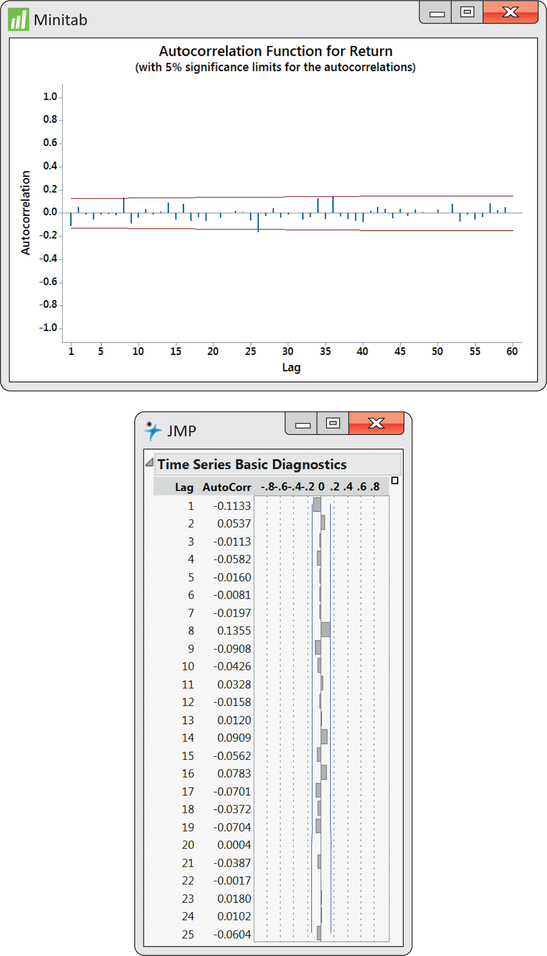
EXAMPLE 13.6 ACF for Disney Returns

ACF outputs from Minitab and JMP are given in Figure 13.10. Notice that the first autocorrelation is plotted negative while the second autocorrelation is plotted positive. From the JMP output, we see that the first two autocorrelations are reported to be −0.1133 and 0.0537, which are basically the values shown in Figure 13.9.⁴

What we also find with the ACF is a band of lines superimposed symmetrically around the 0 correlation value. These lines serve as a test of the significance of the autocorrelations. If a process is truly random, the underlying process autocorrelation at any lag is theoretically 0. However, as we have learned throughout the book, sample statistics (in this case, sample autocorrelations) are subject to sampling variation.

The lines seen on the ACF attempt to incorporate sampling variability of the autocorrelation statistic. In particular, if the underlying autocorrelation at a particular lag is truly 0, then with repeated samples from the process, we would expect 95% of the lag sample autocorrelations to fall within the band limits. Therefore, for any given lag, the limits are an implementation of a 5% level significance test of the null hypothesis that the underlying process autocorrelation is zero. We see from Figure 13.10 that none of the sample autocorrelations breach the limits. The ACF leaves us with no suspicion against randomness, which confirms both our initial visual inspection of the time series with Figure 13.3 (page 646) and the results of the runs test in Example 13.2 (pages 649–650).

654