EXAMPLE 13.8 Simulating Random walks

Consider a simple version of the random walk with , which gives the following equation for the random walk process:

This equation implies that the observed value of at period is simply the observed value of at period plus a random deviation. Let us assume for our study that the error deviations follow the standard Normal distribution, that is, . Furthermore, we start the time series at .

Because the error deviation distribution is symmetrically centered on 0, there is a 50% chance of a deviation being positive or negative. This implies that there is a 50% chance that the variable will increase or decrease from one period to the next. In that light, how might the random walk process evolve over time? It would seem the equal chance of going up or down from period to period will result that random walk observations hovering close to the initial value of 0.

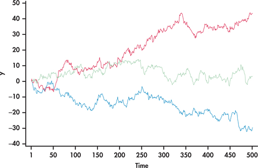
Figure 13.13 shows three simulation runs of our random walk setting for 500 consecutive periods. Notice first that the simulated series look remarkably like stock market charts. In one case (blue line), the random walk series takes a nose dive downward with no indication of returning back. The second case (red line), on the other hand, takes off with the observations steadily increasing. Finally, in the third case (green line), the series wanders around the 0 value. With the first two cases, it would be incorrect to conclude that the processes will continue to trend in the same direction. Moving into the future from , the three random walks can move in any direction, as they did starting from the first period.

659