EXAMPLE 4.41 Portfolio Analysis
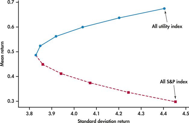
CASE 4.3 By doing the mean computations of Example 4.34 (pages 227–228) and the standard deviation computations of Example 4.40 for different mixes, we find the following values.
| S&P 500 proportion | μR | σR |
|---|---|---|
| 0.0 | 0.675 | 4.403 |
| 0.1 | 0.637 | 4.201 |
| 0.2 | 0.600 | 4.038 |
| 0.3 | 0.562 | 3.919 |
| 0.4 | 0.524 | 3.848 |
| 0.5 | 0.487 | 3.828 |
| 0.6 | 0.449 | 3.860 |
| 0.7 | 0.411 | 3.942 |
| 0.8 | 0.373 | 4.071 |
| 0.9 | 0.336 | 4.243 |
| 1.0 | 0.298 | 4.453 |
From Figure 4.19, we see that the plot of the portfolio mean returns against the corresponding standard deviations forms a parabola. The point on the parabola where the portfolio standard deviation is lowest is the minimum variance portfolio (MVP). From the preceding table, we see that the MVP is somewhere near a 50/50 allocation between the two investments. The solid curve of the parabola provides the preferable options in that the expected return is, for a given level of risk, higher than the dashed line option.
minimum variance portfolio
