Chapter 9 AppendixInference for Categorical Data with Excel, JMP, Minitab, SPSS, CrunchIt!, R, and TI-83/-84 Calculators
Inference for Two-Way Tables
Most of the software packages (except Excel and TI calculators) want the data for the two-way table entered in the following format:
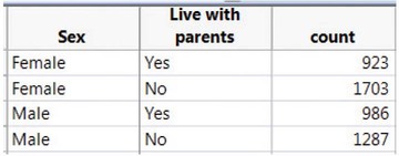

- Enter the data as a two-way table (the layout used in the text).
- Compute the expected counts as (row total × column total)/table total into another two-way table in the spreadsheet. (You can use the Sum(xx:yy) function to find the appropriate totals.)
- Formulas ➔ More functions ➔ Statistical ➔ CHISQ.TEST. Specify the range of cells for both the observed and expected counts.
For a video that shows how to use Excel and the formulas with an example, see the Excel Video Technology Manual: Chi-Square Two-Way Test.

- Enter the data as shown above.
- Analyze ➔ Fit Y by X
- Select and enter the two categorical variables as the response variable and factor variable, and the counts as Weights. Even if there is a clear explanatory/response relationship in the data, which variable takes on which role here is really unimportant, but the “response” will become the column variable in the two-way table.
- Click “OK.”
For a video that shows how to use JMP here with an example, see the JMP Video Technology Manual: Chi-Square Two-Way Test.

- Enter the data as shown above.
- Stat ➔ Tables ➔ Cross-Tabulation and Chi-square
- Select one of the two categorical variables to display as the row variable and the other as the column variable. Select the “Counts” variable to be the “Frequencies” variable.
- Click “Chi-Square.” Click to check the box labeled “Chi-square test.” Check other boxes to display other statistics as desired.
For more information and an example, see the Minitab Video Technology Manual: Chi-Square Two-Way Test.

- Enter the data as shown on page TA9-1. (SPSS really wants individual case data, but that is impractical, as all data you should encounter with this text is summarized.)
- Data ➔ Weight Cases. Select to “Weight cases by” the count variable, then click “OK.”
- Analyze ➔ Descriptive Statistics ➔ Crosstabs. Select one of the categorical variables to be the row variable and the other for columns.
- Click “Statistics.” Check the box for the “Chi-square,” then “Continue.”
- If you want SPSS to display the expected counts, click “Cells” and check the box for them. Click “Continue” and “OK” to perform the test.
For more information and an example, see the SPSS Video Technology Manual: Chi-Square Two-Way Test. The example with summarized data starts about 3:10 into the video (the preceding portion is for raw data).

- Enter the data as shown on page TA9-1 (or open a supplied data file).
- Statistics ➔ Contingency Table ➔ with counts (unless you have raw data, which is very unlikely).
- Select one categorical variable for rows, the second to be the column variable, and the third with the observed counts.
- Click “Calculate.”
For more information (and an example), see the Crunchit! Help Video: Chi-Square Two-Way Test.

- Press 2ndX−1
 for the Matrix Edit Menu. Select a matrix (usually [A]) in which to enter the observed counts.
 - Enter the number of rows, ENTER, and the number of columns in the two-way table. Press ENTER to move to the matrix itself and enter the table counts, pressing ENTER after each to move across the columns and then down the rows. Press 2nd MODE = Quit to exit the editor.
- Press STAT
for the Tests menu, then select option C:χ2-Test. If needed, press 2ndX−1 to change the matrix names for the observed and expected counts. Press ENTER on Calculate.
For more information and an example, see the TI-83/-84 Video Technology Manual: Chi-Square Two-Way Test.

With raw data, use the table function to create a table:
> Table (datasetname) -> twoway.name
where “name” is a name you give the table.
Follow that with
> chisq.test(twoway.name)
With summarized data, use the command
> xtabs (Count ~ rowvar + colvar) -> twoway.name
where those are the variables to be treated as rows (or columns) of the output matrix).
Follow this with
> chisq.test(twoway.name)
In either case, to see the expected counts, use the command
> results$exp
For more information and an example, see the R Video Technology Manual: Chi-Square Two-Way Test.
Goodness of Fit
- Enter the category names in a column (say, A), the observed counts in a column (say, B), and the given probabilities in a column (say, C).
Place the cursor in an empty cell (say, B15) and sum the observed counts using the command
= sum(B1:Bn)
where n is the last row of counts.
Compute the expected counts by placing the cursor at the top of an empty column (say, D) using the command
=C1*B$15
- Drag the cursor to copy the command down until all the expected counts have been calculated.
Calculate the parts of the Chi-square statistic by placing the cursor at the top of a new column (say, E) using the command
=(B1-D1)^2/D1
- Drag the cursor to copy the command down until all the chi-square parts have been calculated.
Sum the parts for the statistic.
=sum(E1:En)
- Formulas ➔ More Functions ➔ Statistical ➔ CHISQ.DIST.RT
- Enter the statistic just calculated and the degrees of freedom (categories – 1). Click “OK” for the P-value.
- Enter the category names in one column and the observed counts in another.
- Analyze ➔ Distribution
- Select and enter the categorical variable as Y and the counts as Freq.
- Click “OK.”
- Click on the red triangle by the variable name and select “Test Probabilities.”
- Enter the given category probabilities. Click “Done.” Two slightly different Chisquare statistics and P-values will be displayed. You are interested in the one labeled “Pearson.”
For a video that shows how to use JMP here with an example, see the JMP Video Technology Manual: Chi-Square GOF Test.
- Enter the category names in one column and the observed counts in another, and the given probabilities in a third.
- Stat ➔ Tables ➔ Chi-square Goodness-of-Fit Test (One Variable)
- Click to enter the column with the observed counts, and the column with the category names. Select the radio button for Specific Proportions and click to enter the column with the given probabilities. Click “OK.”
Minitab’s default is to provide two charts: the first is a bar graph of contributions to the chi-square statistic; the second compares observed and expected counts. If you do not want to see those, click “Graphs” and uncheck the boxes.
For more information and an example, see the Minitab Video Technology Manual: Chi-square GOF Test.
- Enter the category names in one column, the observed counts in another, and the given probabilities in a third.
- Obtain the sum of the observed counts: Analyze ➔ Descriptive Statistics ➔ Frequencies. Click to enter the observed counts as the variable. Click “Statistics” and check the box for “Sum.” Click “Continue” and “OK.” We’ll call the obtained value of the sum Tot.
- Transform ➔ Compute Variable. Enter a new variable name. Compute the parts of the Chi-square statistic as (Observed−Tot*Prob)^2/(Tot*Prob).
- Analyze ➔ Descriptive Statistics ➔ Frequencies. Click to enter the variable just calculated (the parts of the chi-square) as the variable. Obtain the sum; this is the value of the test statistic.
- Transform ➔ Compute Variable. Enter a new variable name and clear the old formula. In the Function group box, select “CDF and Noncentral CDF.” Doubleclick “CDF.Chisq” to transfer that shell into the formula box. Enter the value of the test statistic just obtained and the degrees of freedom (categories – 1). Click “OK.” That result is the P-value of the test.
- Enter the category names in one column and the observed counts in another.
- If the null hypothesis is that all categories are equally likely, there is no need for a column of hypothesized probabilities; otherwise, enter those in a third column.
- Statistics ➔ Chi-squared Goodness-of-Fit
- Click to enter the column of observed counts and the column of hypothesized probabilities (if there is one). Click “Calculate.”
For more information (and an example), see the Crunchit! Help Video: Chi-Square Goodness of Fit Test.
- Use the Statistics List Editor (STAT ENTER) to enter a list of observed counts and a list of hypothesized probabilities (say, L1=observed and L2=probabilities).
- STAT
ENTER for 1-VarStats. Enter the name of the list with the observed counts. The statistic labeled ∑x is the total sample size. In the next step, that is referred to as Tot.
- Calculate a list of expected counts by placing the cursor in the header of an empty list (L3, say). Enter the formula Tot*L2.
- If you have a TI-84, press STAT
for the TESTS menu and then arrow down (or up) to option D:χ2GOF-Test. Enter the list names for the observed and expected counts and the degrees of freedom (categories – 1). Press ENTER for the results.
- If you have a TI-83, calculate the parts of the chi-square test statistic by placing the cursor in the header of a cleared list (say, L4) and enter the formula (L1−L3)^2/L3 and press ENTER .
- Obtain the chi-square statistic by summing L4 as above.
Obtain the P-value: 2ndVARS8 gives the χ2CDF shell. Enter the test statistic value just obtained, infinity, and the degrees of freedom (categories – 1) separated by commas. Practically speaking, any “large” positive number will work as infinity. An example of the command with 4 categories is shown below.
χ2CDF(2.345,99999,3)
For more information and an example, see the TI Video Technology Manual: Chi-square GOF Test.
- Enter variable of observed counts and a variable of hypothesized probabilities.
Use chisq.test(obs,p=probs) to perform the test. An example is shown below.
> act<-c(15,25,40,60)
> pr<-c(0.1,0.2,0.3,0.4)
> chisq.test(act,p=pr)
Chi-squared test for given probabilities
data: act
X-squared = 0.7738, df = 3, p-value = 0.8557
For more information and an example, see the R Video Technology Manual: Chi-square Goodness of Fit Test.