10.3 Some Details of Regression Inference
We have assumed that you will use software to handle regression in practice. If you do, it is much more important to understand what the standard error of the slope SEb1 means than it is to know the formula your software uses to find its numerical value. For that reason, we have not yet given formulas for the standard errors. We have also not explained the block of output from software that is labeled ANOVA or Analysis of Variance. This section addresses both of these omissions.
Standard errors
We give the formulas for all the standard errors we have met, for two reasons. First, you may want to see how these formulas can be obtained from facts you already know. The second reason is more practical: some software (in particular, spreadsheet programs) does not automate inference for prediction. We see that the hard work lies in calculating the regression standard error s, which almost any regression software will do for you. With s in hand, the rest is straightforward, but only if you know the details.
Tests and confidence intervals for the slope of a population regression line start with the slope b1 of the least-squares line and with its standard error SEb1. If you are willing to skip some messy algebra, it is easy to see where SEb1 and the similar standard error SEb0 of the intercept come from.
- The regression model takes the explanatory values xi to be fixed numbers and the response values yi to be independent random variables all having the same standard deviation σ.
- The least-squares slope is b1=rsy/sx. Here is the first bit of messy algebra that we skip: it is possible to write the slope b1 as a linear function of the responses, b1=∑aiyi. The coefficients ai depend on the xi.
- Because the ai are constants, we can find the variance of b1 by applying the rule for the variance of a sum of independent random variables. It is just σ2∑a2i. A second piece of messy algebra shows that this simplifies to
σ2b1=σ2∑(xi−ˉx)2

The standard deviation σ about the population regression line is, of course, not known. If we estimate it by the regression standard error s based on the residuals from the least-squares line, we get the standard error of b1. Here are the results for both slope and intercept.
Standard Errors for Slope and Intercept
The standard error of the slope b1 of the least-squares regression line is
SEb1=s√∑(xi−ˉx)2
The standard error of the intercept b0 is
SEb0=s√1n+ˉx2∑(xi−ˉx)2
The critical fact is that both standard errors are multiples of the regression standard error s. In a similar manner, accepting the results of yet more messy algebra, we get the standard errors for the two uses of the regression line that we have studied.
Standard Errors for Two Uses of the Regression Line
The standard error for estimating the mean response when the explanatory variable x takes the value x* is
SEˆμ=s√1n+(x*−ˉx)2∑(xi−ˉx)2
The standard error for predicting an individual response when x=x* is
SEˆy=s√1+1n+(x*−ˉx)2∑(xi−ˉx)2=√SE2ˆμ+s2
Once again, both standard errors are multiples of s. The only difference between the two prediction standard errors is the extra 1 under the square root sign in the standard error for predicting an individual response. This added term reflects the additional variation in individual responses. It means that, as we have said earlier, SEˆy is always greater than SEˆμ.
EXAMPLE 10.11 Prediction Intervals from a Spreadsheet
In Example 10.7 (pages 511–512), we used statistical software to predict the log income of Alexander, who has EDUC=16 years of education. Suppose that we have only the Excel spreadsheet. The prediction interval then requires some additional work.
Step 1. From the Excel output in Figure 10.5 (page 492), we know that s=1.1146. Excel can also find the mean and variance of the EDUC x for the 100 entrepreneurs. They are ˉx=13.28 and s2x=5.901.
Step 2. We need the value of ∑(xi−ˉx)2. Recalling the definition of the variance, we see that this is just
∑(xi−ˉx)2=(n−1)s2x=(99)(5.901)=584.2
Step 3. The standard error for predicting Alexander’s log income from his years of education, x*=16, is
SEˆy=s√1+1n+(x*−ˉx)2∑(xi−ˉx)2=1.1146√1+1100+(16−13.28)2584.2=1.1146√1+1100+7.3984584.2=(1.1146)(1.01127)=1.12716
Step 4. We predict Alexander’s log income from the least-squares line (Figure 10.5 again):
ˆy=8.2546+(0.1126)(16)=10.0562
This agrees with the “Fit” from software in Example 10.8. The 95% prediction interval requires the 95% critical value for t(98). For hand calculation we use t*=1.990 from Table D with df=80. The interval is
ˆy±t*SEˆy=10.0562±(1.990)(1.12716)=10.0562±2.2430=7.8132to12.2992
This agrees with the software result in Example 10.8, with a small difference due to roundoff and especially to not having the exact t*.
The formulas for the standard errors for prediction show us one more thing about prediction. They both contain the term (x*−ˉx)2, the squared distance of the value x* for which we want to do prediction from the mean ˉx of the x-values in our data. We see that prediction is most accurate (smallest margin of error) near the mean and grows less accurate as we move away from the mean of the explanatory variable. If you know what values of x you want to do prediction for, try to collect data centered near these values.
Apply Your Knowledge
Question 10.55
10.55 T-bills and inflation.
Figure 10.10 (page 499) gives the Excel output for regressing the annual return on Treasury bills on the annual rate of inflation. The data appear in Table 10.1 (page 498). Starting with the regression standard error s=2.1407 from the output and the variance of the inflation rates in Table 10.1 (use your calculator), find the standard error of the regression slope SEb1. Check your result against the Excel output.
10.55
SEb1=0.0993. It is the same as the Excel output.
Question 10.56
10.56 Predicting T-bill return.
Figure 10.16 (page 514) uses statistical software to predict the return on Treasury bills in a year when the inflation rate is 2.25%. Let’s do this without specialized software. Figure 10.10 (page 499) contains Excel regression output. Use a calculator or software to find the variance s2x of the annual inflation rates in Table 10.1 (page 498). From this information, find the 95% prediction interval for one year’s T-bill return. Check your result against the software output in Figure 10.16.
Analysis of variance for regression
Software output for regression problems, such as those in Figures 10.5, 10.6, and 10.10 (pages 492,493, and 499), reports values under the heading of ANOVA or Analysis of Variance. You can ignore this part of the output for simple linear regression, but it becomes useful in multiple regression, where several explanatory variables are used together to predict a response.
analysis of variance
Analysis of variance (ANOVA) is the term for statistical analyses that break down the variation in data into separate pieces that correspond to different sources of variation. In the regression setting, the observed variation in the responses yi comes from two sources:
- As the explanatory variable x moves, it pulls the response with it along the regression line. In Figure 10.4 (page 487), for example, entrepreneurs with 15 years of education generally have higher log incomes than those entrepreneurs with nine years of education. The least-squares line drawn on the scatterplot describes this tie between x and y.
- When x is held fixed, y still varies because not all individuals who share a common x have the same response y. There are several entrepreneurs with 11 years of education, and their log income values are scattered above and below the least-squares line.
We discussed these sources of variation in Chapter 2, where the main point was that the squared correlation r2 is the proportion of the total variation in the responses that comes from the first source, the straight-line tie between x and y.
ANOVA equation
Analysis of variance for regression expresses these two sources of variation in algebraic form so that we can calculate the breakdown of overall variation into two parts. Skipping quite a bit of messy algebra, we just state that this analysis of variance equation always holds:
total variation in y=variation along the line+variation about the line∑(yi−ˉy)2=∑(ˆyi−ˉy)2+∑(yi−ˆyi)2
Understanding the ANOVA equation requires some thought. The “total variation” in the responses yi is expressed by the sum of the squares of the deviations yi−ˉy. If all responses were the same, all would equal the mean response ˉy, and the total variation would be zero. The total variation term is just n−1 times the variance of the responses. The “variation along the line” term has the same form: it is the variation among the predicted responses ˆyi. The predicted responses lie on the least-squares line—they show how y moves in response to x. The “variation about the line” term is the sum of squares of the residuals yi−ˆyi. It measures the size of the scatter of the observed responses above and below the line. If all the responses fell exactly on a straight line, the residuals would all be 0 and there would be no variation about the line. The total variation would equal the variation along the line.
EXAMPLE 10.12 ANOVA for Entrepreneurs’ Log Income
entre
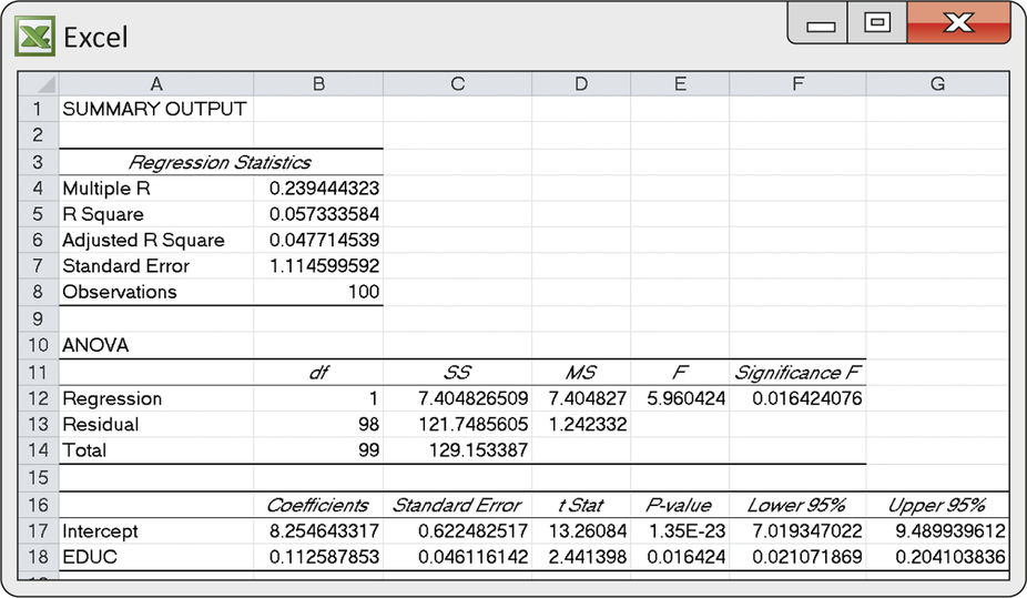
CASE 10.1 Figure 10.18 repeats Figure 10.5. It is the Excel output for the regression of log income on years of education (Case 10.1). The three terms in the analysis of variance equation appear under the “SS” heading. SS stands for sum of squares, reflecting the fact that each of the three terms is a sum of squared quantities. You can read the output as follows:
total variation iny=variation along the line+variation about the linetotal SS=regression SS+residual SS129.1534=7.4048+121.7486
sum of squares
The proportion of variation in log incomes explained by regressing years of education is
r2=Regression SSTotal SS=7.4048129.1534=0.0573
This agrees with the “R Square” value in the output. Only about 6% of the variation in log incomes is explained by the linear relationship between log income and years of education. The rest is variation in log incomes among entrepreneurs with similar levels of education.
degrees of freedom
There is more to the ANOVA table in Figure 10.18. Each sum of squares has a degrees of freedom. The total degrees of freedom are n−1=99, the degrees of freedom for the variance of n=100 observations. This matches the total sum of squares, which is the sum of squares that appears in the definition of the variance. We know that the degrees of freedom for the residuals and for t statistics in simple linear regression are n−2. Therefore, it is no surprise that the degrees of freedom for the residual sum of squares are also n−2=98. That leaves just 1 degree of freedom for regression, because degrees of freedom in ANOVA also add:
Total df=Regression df+Residual dfn−1=1+n−2
mean square
Dividing a sum of squares by its degrees of freedom gives a mean square (MS). The total mean square (not given in the output) is just the variance of the responses yi. The residual mean square is the square of our old friend the regression standard error:
Residual mean square=Residual SSResidual df=∑(yi−ˆyi)2n−2=s2
You see that the analysis of variance table reports in a different way quantities such as r2 and s that are needed in regression analysis. It also reports in a different way the test for the overall significance of the regression. If regression on x has no value for predicting y, we expect the slope of the population regression line to be close to zero. That is, the null hypothesis of “no linear relationship” is H0:β1=0. To test H0, we standardize the slope of the least-squares line to get a t statistic. The ANOVA approach starts instead with sums of squares. If regression on x has no value for predicting y, we expect the regression SS to be only a small part of the total SS, most of which will be made up of the residual SS. It turns out that the proper way to standardize this comparison is to use the ratio
F=Regression MSResidual MS
ANOVA F statistic
This ANOVA F statistic appears in the second column from the right in the ANOVA table in Figure 10.18. If H0 is true, we expect F to be small. For simple linear regression, the ANOVA F statistic always equals the square of the t statistic for testing H0:β1=0. That is, the two tests amount to the same thing.
EXAMPLE 10.13 ANOVA for Entrepreneurs’ Log Income, Continued
The Excel output in Figure 10.18 (page 521) contains the values for the analysis of variance equation for sums of squares and also the corresponding degrees of freedom. The residual mean square is
Residual MS=Residual SSResidual df=121.748698=1.2423
The square root of the residual MS is √1.2423=1.1146. This is the regression standard error s, as claimed. The ANOVA F statistic is
F=Regression MSResidual MS=7.40481.2423=5.9604
The square root of F is √5.9604=2.441. Sure enough, this is the value of the t statistic for testing the significance of the regression, which also appears in the Excel output. The P-value for F,P=0.0164, is the same as the two-sided P-value for t.
We have now explained almost all the results that appear in a typical regression output such as Figure 10.18. ANOVA shows exactly what r2 means in regression. Aside from this, ANOVA seems redundant; it repeats in less clear form information that is found elsewhere in the output. This is true in simple linear regression, but ANOVA comes into its own in multiple regression, the topic of the next chapter.
Apply Your Knowledge
T-bills and inflation. Figure 10.10 (page 499) gives Excel output for the regression of the rate of return on Treasury bills against the rate of inflation during the same year. Exercises 10.57 through 10.59 use this output.
Question 10.57
10.57 A significant relationship?
The output reports two tests of the null hypothesis that regressing on inflation does help to explain the return on T-bills. State the hypotheses carefully, give the two test statistics, show how they are related, and give the common P-value.
10.57
H0:β1=0 or no linear relationship, Ha:β1≠0 or there is a linear relationship. t=7.08, F=50.14, F=t2. P-value=3.044E-09.
Question 10.58
10.58 The ANOVA table.
Use the numerical results in the Excel output to verify each of these relationships.
- The ANOVA equation for sums of squares.
- How to obtain the total degrees of freedom and the residual degrees of freedom from the number of observations.
- How to obtain each mean square from a sum of squares and its degrees of freedom.
- How to obtain the F statistic from the mean squares.
Question 10.59
10.59 ANOVA by-products.
- The output gives r2=0.4815. How can you obtain this from the ANOVA table?
- The output gives the regression standard error as s=2.1407. How can you obtain this from the ANOVA table?
10.59
(a) r2=RegressionSS/TotalSS=229.7644/447.2188=0.4815. (b) s=√4.582488=2.141.