11.1 Data Analysis for Multiple Regression


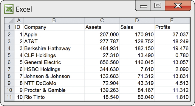
Table 11.1 shows some characteristics of 15 prominent companies that are part of the British Broadcasting Corporation (BBC) Global 30 stock market index, commonly used as a global economic barometer. Included are an identification number, the company name, assets, sales, and profits for the year 2013 (all in billions of U.S. dollars).2 How are profits related to sales and assets? In this case, profits represents the response variable, and sales and assets are two explanatory variables. The variables ID and Company both label each observation.
bbcg30
| ID | Company | Assets ($ billions) | Sales ($ billions) | Profits ($ billions) |
|---|---|---|---|---|
| 1 | Apple | 207.000 | 170.910 | 37.037 |
| 2 | AT&T | 277.787 | 128.752 | 18.249 |
| 3 | Berkshire Hathaway | 484.931 | 182.150 | 19.476 |
| 4 | CLP Holdings | 27.310 | 13.490 | 0.780 |
| 5 | General Electric | 656.560 | 146.045 | 13.057 |
| 6 | HSBC Holdings | 344.630 | 7.610 | 2.090 |
| 7 | Johnson & Johnson | 132.683 | 71.312 | 13.831 |
| 8 | NTT DoCoMo | 72.904 | 43.319 | 4.513 |
| 9 | Procter & Gamble | 139.263 | 84.167 | 11.312 |
| 10 | Rio Tinto | 18.540 | 86.040 | 1.810 |
| 11 | SAP | 37.334 | 23.170 | 4.582 |
| 12 | Siemens | 136.250 | 101.340 | 5.730 |
| 13 | Southern Company | 64.546 | 17.087 | 1.710 |
| 14 | Wal-Mart Stores | 204.751 | 476.294 | 16.022 |
| 15 | Woodside Petroleum | 22.040 | 5.530 | 1.620 |
Data for multiple regression
The data for a simple linear regression problem consist of observations on an explanatory variable x and a response variable y. We use n for the number of cases. The major difference in the data for multiple regression is that we have more than one explanatory variable.
EXAMPLE 11.5 Data for Assets, Sales, and Profits
CASE 11.1 In Case 11.1, the cases are the 15 companies. Each observation consists of a value for a response variable (profits) and values for the two explanatory variables (assets and sales).
In general, we have data on n cases and we use p for the number of explanatory variables. Data are often entered into spreadsheets and computer regression programs in a format where each row describes a case and each column corresponds to a different variable.
EXAMPLE 11.6 Spreadsheet Data for Assets, Sales, and Profits
CASE 11.1 In Case 11.1, there are 15 companies; assets and sales are the explanatory variables. Therefore, n=15 and p=2. Figure 11.1 shows the part of an Excel spreadsheet with the first 10 cases.
Apply Your Knowledge
Question 11.3
11.3 Assets, interest-bearing deposits, and equity capital.
Table 11.2 gives data for insured commercial banks, by state or other area.3 The cases are the 50 states, the District of Columbia, Guam, and Puerto Rico. Bank assets, interest-bearing deposits, and equity capital are given in billions of dollars. We are interested in describing how assets are explained by total interest-bearing deposits and total equity capital.
- What is the response variable?
- What are the explanatory variables?
- What is p, the number of explanatory variables?
- What is n, the sample size?
- Is there a label variable? If yes, identify it.
11.3
(a) Assets. (b) Total interest-bearing deposits and total equity capital. (c) p=2. (d) n=53. (e) The label variable is State or Area.
banks
Question 11.4
11.4 Describing a multiple regression.
As part of a study, data from 55 Fortune 500 companies were obtained.4 Based on these data, the researchers described the relationship between a company’s annual profits and the age and facial width-to-height ratio of its CEO.
- What is the response variable?
- What is n, the number of cases?
- What is p, the number of explanatory variables?
- What are the explanatory variables?
Preliminary data analysis for multiple regression
As with any statistical analysis, we begin our multiple regression analysis with a careful examination of the data. We look first at each variable separately, then at relationships among the variables. In both cases, we continue our practice of combining plots and numerical descriptions.
| State or area | Assets | Deposits ($ billions) |
Equity ($ billions) |
State or area | Assets | Deposits ($ billions) |
Equity ($ billions) |
|---|---|---|---|---|---|---|---|
| Alabama | 230.6 | 131.6 | 32.3 | Montana | 26.4 | 16.0 | 3.1 |
| Alaska | 5.1 | 2.2 | 0.7 | Nebraska | 57.5 | 36.6 | 5.9 |
| Arizona | 18.7 | 11.4 | 1.9 | Nevada | 21.1 | 7.8 | 5.1 |
| Arkansas | 62.2 | 42.9 | 7.4 | New Hampshire | 3.3 | 2.3 | 0.3 |
| California | 548.8 | 294.2 | 70.3 | New Jersey | 54.2 | 34.0 | 5.5 |
| Colorado | 43.5 | 28.5 | 4.1 | New Mexico | 15.4 | 9.7 | 1.7 |
| Connecticut | 25.8 | 15.4 | 2.6 | New York | 749.9 | 418.4 | 85.7 |
| Delaware | 1005.0 | 582.0 | 140.8 | North Carolina | 1696.7 | 866.2 | 208.6 |
| District of Columbia | 2.0 | 1.2 | 0.2 | North Dakota | 23.4 | 15.9 | 2.2 |
| Florida | 126.4 | 82.2 | 14.3 | Ohio | 2687.3 | 1334.4 | 254.3 |
| Georgia | 266.7 | 160.0 | 32.0 | Oklahoma | 84.6 | 57.3 | 8.1 |
| Guam | 1.7 | 1.2 | 0.1 | Oregon | 19.1 | 11.6 | 2.7 |
| Hawaii | 37.7 | 22.6 | 4.4 | Pennsylvania | 145.1 | 95.3 | 17.8 |
| Idaho | 5.9 | 3.5 | 0.7 | Rhode Island | 101.2 | 53.2 | 16.3 |
| Illinois | 375.9 | 230.8 | 40.9 | South Carolina | 35.7 | 23.8 | 3.7 |
| Indiana | 62.7 | 42.2 | 6.9 | South Dakota | 2786.7 | 1636.0 | 293.2 |
| Iowa | 69.0 | 46.7 | 7.1 | Tennessee | 82.4 | 53.8 | 9.4 |
| Kansas | 51.8 | 34.6 | 5.7 | Texas | 358.8 | 195.1 | 40.2 |
| Kentucky | 53.8 | 36.3 | 5.9 | Utah | 394.3 | 285.7 | 50.7 |
| Louisiana | 54.5 | 35.1 | 5.9 | Vermont | 4.1 | 2.8 | 0.4 |
| Maine | 23.3 | 19.1 | 2.1 | Virginia | 563.1 | 330.0 | 69.4 |
| Maryland | 25.6 | 16.0 | 2.7 | Washington | 59.9 | 36.0 | 7.6 |
| Massachusetts | 292.6 | 153.2 | 24.1 | West Virginia | 27.9 | 18.6 | 3.1 |
| Michigan | 44.8 | 30.0 | 4.8 | Wisconsin | 83.0 | 53.5 | 9.9 |
| Minnesota | 59.5 | 39.7 | 6.2 | Wyoming | 6.5 | 4.5 | 0.6 |
| Mississippi | 75.6 | 46.9 | 8.7 | Puerto Rico | 67.6 | 41.1 | 8.0 |
| Missouri | 129.6 | 82.1 | 12.9 |
EXAMPLE 11.7 Describing Assets, Sales, and Profits
bbcg30
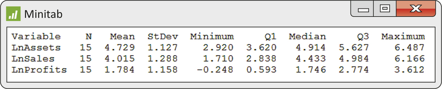
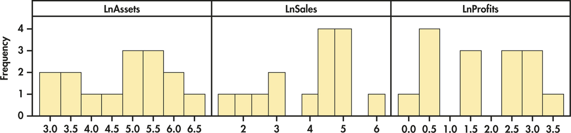
CASE 11.1 A quick scan of the data in Table 11.1 (page 534) using boxplots or histograms suggests each variable is strongly skewed to the right. It is common to use logarithms to make economic and financial data more symmetric before doing inference as it pulls in the long tail of a skewed distribution, thereby reducing the possibility of influential observations. Figure 11.2 shows descriptive statistics for these transformed values, and Figure 11.3 presents the histograms. Each distribution appears relatively symmetric (mean and median of each transformed variable are approximately equal) with no obvious outliers.

Later in this chapter, we describe a statistical model that is the basis for inference in multiple regression. This model does not require Normality for the distributions of the response or explanatory variables. The Normality assumption applies to the distribution of the residuals, as was the case for inference in simple linear regression. We look at the distribution of each variable to be used in a multiple regression to determine if there are any unusual patterns that may be important in building our regression analysis.
Apply Your Knowledge
Question 11.5
11.5 Is there a problem?
Refer to Exercise 11.4 (page 535). The 55 firms in the sample represented a range of industries, including retail and computer manufacturing. Suppose this resulted in the response variable, annual profits, having a bimodal distribution (see page 56 for a trimodal distribution). Considering that this distribution is not Normal, will this necessarily be a problem for inference in multiple regression? Explain your answer.
11.5
No. Multiple regression does not require the response to be Normally distributed, only the residuals need to be Normally distributed.
Question 11.6
11.6 Look at the data.
Examine the data for assets, deposits, and equity given in Table 11.2. That is, use graphs to display the distribution of each variable. Based on your examination, how would you describe the data? Are there any states or other areas that you consider to be outliers or unusual in any way? Explain your answer.
banks
Now that we know something about the distributions of the individual variables, we look at the relations between pairs of variables.
EXAMPLE 11.8 Assets, Sales, and Profits in Pairs
bbcg30
CASE 11.1 With three variables, we also have three pairs of variables to examine. Figure 11.4 gives the three correlations, and Figure 11.5 displays the corresponding scatterplots. We used a scatterplot smoother (page 68) to help us see the overall pattern of each scatterplot.
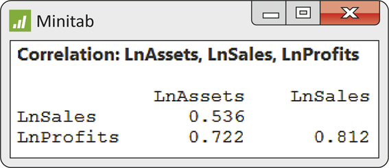
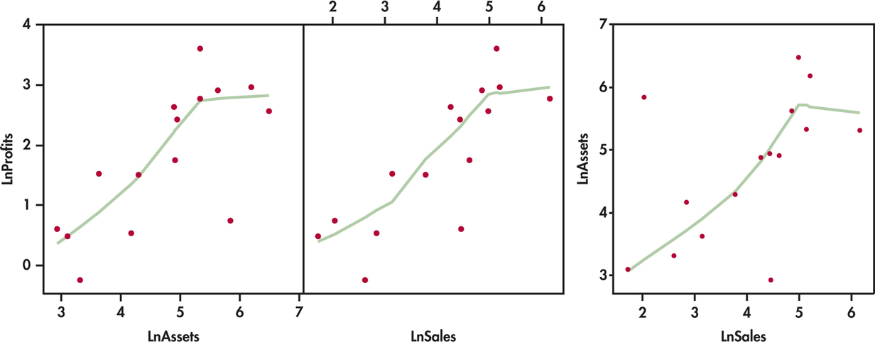
On the logarithmic scale, both assets and sales have reasonably strong positive correlations with profits. These variables may be useful in explaining profits. Assets and sales are positively correlated (r=0.536) but not as strongly. Because we will use both assets and sales to explain profits, we would be concerned if this correlation were high. Two highly correlated explanatory variables contain about the same information, so both together may explain profits only a little better than either alone.
The plots are more revealing. The relationship between profits and each of the two explanatory variables appears reasonably linear. Apple has high profits relative to both sales and assets, creating a kink in the smoothed curve. The relationship between assets and sales is also relatively linear. There are two companies, HSBC Holdings and Rio Tinto, with unusual combinations of assets and sales. HSBC Holdings has far less profits and sales than would be predicted by assets alone. On the other hand, these profits are well predicted using sales alone. Similarly, Rio Tinto has far less profits and assets than would be predicted by sales alone, but profits are well predicted using assets alone. This suggests that both variables may be helpful in predicting profits. The portion of profits that is unexplained by one explanatory variable is explained by the other.
Apply Your Knowledge
Question 11.7
11.7 Examining the pairs of relationships.
Examine the relationship between each pair of variables in Table 11.2 (page 536). That is, compute correlations and construct scatterplots. Based on these summaries, describe these relationships. Are there any states or other areas that you consider unusual in any way? Explain your answer.
11.7
Correlations are 0.9959, 0.9915, and 0.9912. All the plots show a strong relationship between the two variables, but it is not quite linear because there is some curvature in each of the plots. Additionally, four states stick out on all plots: Delaware, North Carolina, Ohio, and South Dakota.
banks
Question 11.8
11.8 Try logs.
The data file for Table 11.2 also contains the logarithms of each variable. Find the correlations and generate scatterplots for each pair of transformed variables. Interpret the results and then compare with your analysis of the original variables.
banks
Estimating the multiple regression coefficients
Simple linear regression with a response variable y and one explanatory variable x begins by using the least-squares idea to fit a straight line ˆy=b0+b1x to data on the two variables. Although we now have p explanatory variables, the principle is the same: we use the least-squares idea to fit a linear function
ˆy=b0+b1x1+b2x2+⋯+bpxp
to the data.

We use a subscript i to distinguish different cases. For the ith case, the predicted response is
ˆyi=b0+b1xi1+b2xi2+⋯+bpxip
As usual, the residual is the difference between the observed value of the response variable and the value predicted by the model:
e=observed response−predicted response
For the ith case, the residual is
ei=yi−ˆyi
The method of least squares chooses the b’s that make the sum of squares of the residuals as small as possible. In other words, the least-squares estimates are the values that minimize the quantity
∑(yi−ˆyi)2
As in the simple linear regression case, it is possible to give formulas for the least-squares estimates. Because the formulas are complicated and hand calculation is out of the question, we are content to understand the least-squares principle and to let software do the computations.
EXAMPLE 11.9 Predicting Profits from Sales and Assets
bbcg30
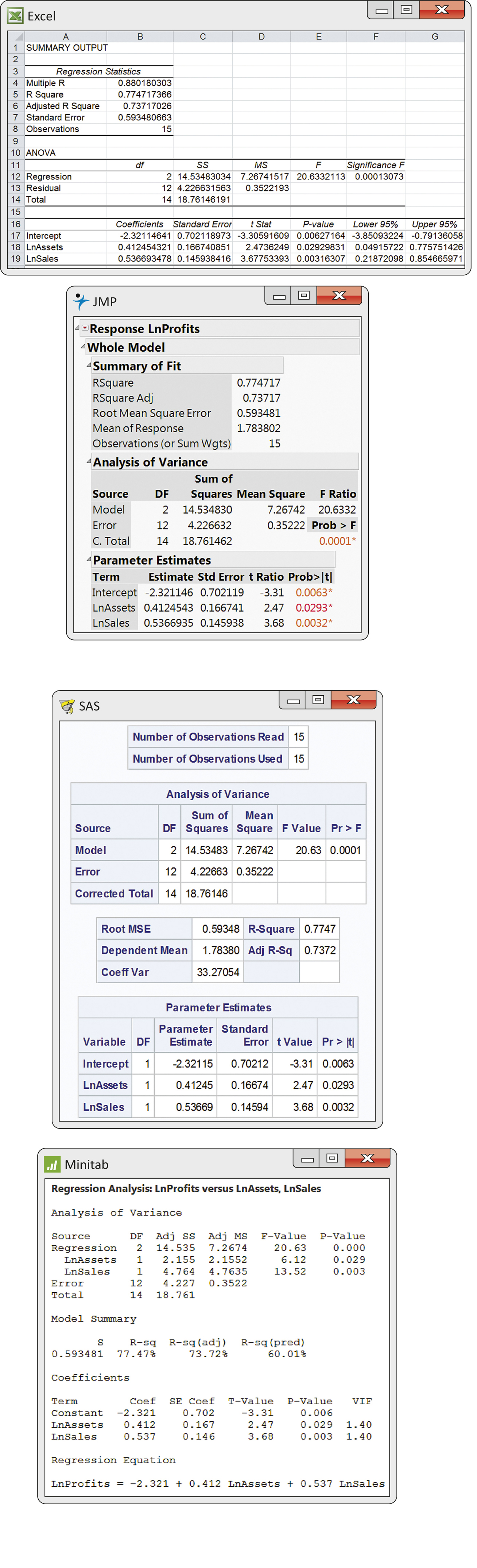
CASE 11.1 Our examination of the logarithm-transformed explanatory and response variables separately and then in pairs did not reveal any severely skewed distributions with outliers or potential influential observations. Outputs for the multiple regression analysis from Excel, JMP, SAS, and Minitab are given in Figure 11.6. Notice that the number of digits provided varies with the software used. Rounding the results to four decimal places gives the least-squares equation
^LnProfits=−2.3211+0.4125×LnAssets+0.5367×LnSales
Apply Your Knowledge
Question 11.9
11.9 Predicting bank assets.
Using the bank data in Table 11.2 (page 536), do the regression to predict assets using deposits and equity capital. Give the least-squares regression equation.
11.9
ˆy=−11.50871+1.38356X1+2.32749X2.
banks
Question 11.10
11.10 Regression after transforming.
In Exercise 11.8 (page 538), we considered the logarithm transformation for all variables in Table 11.2. Run the regression using the logarithm-transformed variables and report the least-squares equation. Note that the units differ from those in Exercise 11.9, so the results cannot be directly compared.
banks
Regression residuals
The residuals are the errors in predicting the sample responses from the multiple regression equation. Recall that the residuals are the differences between the observed and predicted values of the response variable.
e=observed response−predicted response=y−ˆy
As with simple linear regression, the residuals sum to zero, and the best way to examine them is to use plots.
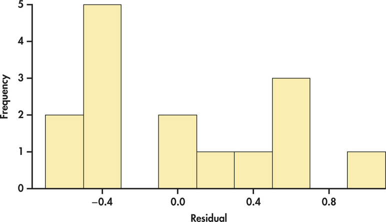
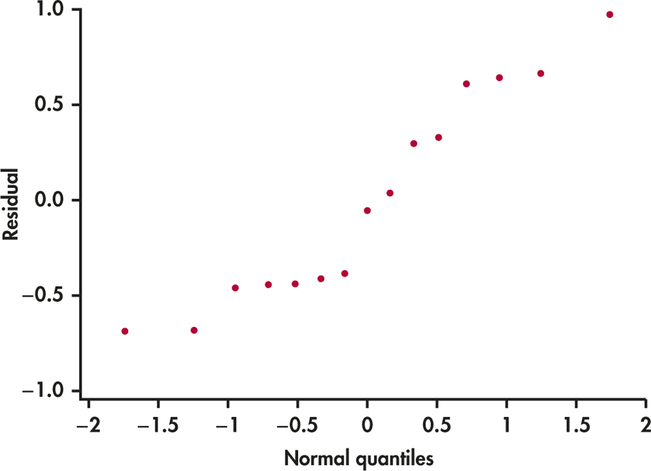
We first examine the distribution of the residuals. To see if the residuals appear to be approximately Normal, we use a histogram and Normal quantile plot.
EXAMPLE 11.10 Distribution of the Residuals
bbcg30
CASE 11.1 Figure 11.7 is a histogram of the residuals. The units are billions of dollars. The distribution does not look symmetric but does not have any outliers. The Normal quantile plot in Figure 11.8 is somewhat linear. Given the small sample size, these plots are not extremely out of the ordinary. Similar to simple linear regression, inference is robust against moderate lack of Normality, so we’re just looking for obvious violations. There do not appear to be any here.
Another important aspect of examining the residuals is to plot them against each explanatory variable. Sometimes, we can detect unusual patterns when we examine the data in this way.
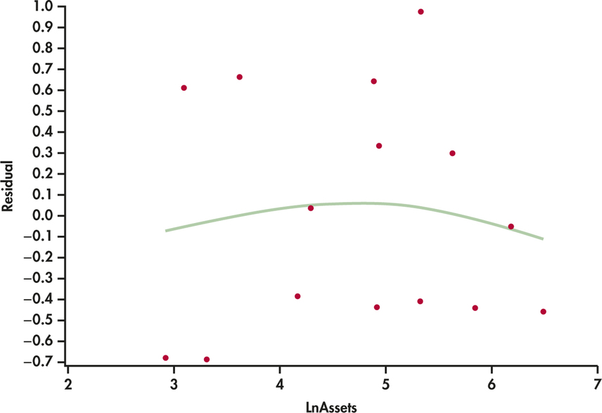
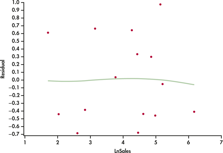
EXAMPLE 11.11 Residual Plots
bbcg30
CASE 11.1 The residuals are plotted versus log assets in Figure 11.9 and versus log sales in Figure 11.10. In both cases, the residuals appear reasonably randomly scattered above and below zero. The smoothed curves suggest a slight curvature in the pattern of residuals versus log assets but not to the point of considering further analysis. We’re likely seeing more in the data than there really is given the small sample size.
Apply Your Knowledge
Question 11.11
11.11 Examine the residuals.
In Exercise 11.9, you ran a multiple regression using the data in Table 11.2 (page 536). Obtain the residuals from this regression and plot them versus each of the explanatory variables. Also, examine the Normality of the residuals using a histogram or stemplot. If possible, use your software to make a Normal quantile plot. Summarize your conclusions.
11.11
The two residual plots show the curvature problem we noted in the previous exercise. The Normal quantile plot shows that the residuals are not Normally distributed because of several outliers on either tail.
banks
Question 11.12
11.12 Examine the effect of Ohio.
The state of Ohio has far more assets than predicted by the regression equation. Delete this observation and rerun the multiple regression. Describe how the regression coefficients change.
banks
Question 11.13
11.13 Residuals for the log analysis.
In Exercise 11.10, you carried out multiple regression using the logarithms of all the variables in Table 11.2. Obtain the residuals from this regression and examine them as you did in Exercise 11.11. Summarize your conclusions and compare your plots with the plots for the original variables.
11.13
The residual plots are much better for the log transformed data; there is no longer any curvature in the plots. The Normal quantile plot shows the data are much better and roughly Normally distributed.
banks
Question 11.14
11.14 Examine the effect of Massachusetts.
For the logarithm-transformed data, Massachusetts has far more assets than predicted by the regression equation. Delete Massachusetts from the data set and rerun the multiple regression using the transformed data. Describe how the regression coefficients change.
banks
The regression standard error
Just as the sample standard deviation measures the variability of observations about their mean, we can quantify the variability of the response variable about the predicted values obtained from the multiple regression equation. As in the case of simple linear regression, we first calculate a variance using the squared residuals:
s2=1n−p−1∑e2i=1n−p−1∑(yi−ˆyi)2
The quantity n−p−1 1 is the degrees of freedom associated with s2. The number of degrees of freedom equals the sample size n minus (p+1), the number of coefficients bi in the multiple regression model. In the simple linear regression case, there is just one explanatory variable, so p=1 and the number of degrees of freedom for s2 is n−2. The regression standard error s is the square root of the sum of squares of residuals divided by the number of degrees of freedom:
s=√s2
Apply Your Knowledge
Question 11.15
CASE 11.111.15 Reading software output.
Regression software usually reports both s2 and the regression standard error s. For the assets, sales, and profits data of Case 11.1 (page 534), the approximate values are s2=0.352 and s=0.593. Locate s2 and s in each of the four outputs in Figure 11.6 (pages 539–541). Give the unrounded values from each output. What name does each software give to s?
11.15
For Minitab: s2=0.3522, s=0.593481; s is called S. For SAS: s2=0.35222, s=0.59348; s is called Root MSE. For JMP: s2=0.35222, s=0.593481; s is called Root Mean Square Error. For Excel: s2=0.3522193, s=0.59348066; s is called Standard Error.
Question 11.16
CASE 11.111.16 Compare the variability.
Figure 11.2 (page 536) gives the standard deviation sy of the log profits of the BBC Global 30 companies. What is this value? The regression standard error s from Figure 11.6 also measures the variability of log profits, this time after taking into account the effect of assets and sales. Explain briefly why we expect s to be smaller than sy. One way to describe how well multiple regression explains the response variable y is to compare s with sy.
Case 11.1 (page 534) uses data on the assets, sales, and profits of 15 companies from the BBC Global 30 index. These are not a simple random sample (SRS) from any population. They are selected and revised by the editors of the BBC from three regions of the world to represent the state of the global economy.
Data analysis does not require that the cases be a random sample from a larger population. Our analysis of Case 11.1 tells us something about these companies—not about all publicly traded companies or any other larger group. Inference, as opposed to data analysis, draws conclusions about a population or process from which our data are a sample. Inference is most easily understood when we have an SRS from a clearly defined population. Whether inference from a multiple regression model not based on a random sample is trustworthy is a matter for judgment.
Applications of statistics in business settings frequently involve data that are not random samples. We often justify inference by saying that we are studying an underlying process that generates the data. For example, in salary-discrimination studies, data are collected on all employees in a particular group. The salaries of these current employees reflect the process by which the company sets salaries. Multiple regression builds a model of this process, and inference tells us whether gender or age has a statistically significant effect in the context of this model.