14.1 One-Way Analysis of Variance
 This page includes Video Technology Manuals
 This page includes Statistical Videos
Which of four advertising offers mailed to sample households produces the highest sales in dollars? Which of six brands of automobile tires wears longest? In each of these settings, we wish to compare several groups or treatments. Also, the data are subject to sampling variability. We would not, for example, expect the same sales data if we mailed the advertising offers to different sets of households. We also would not expect the same tread lifetime data if the tire experiment were repeated under similar conditions.
ANOVA
Because of this variability, we pose the question for inference in terms of the mean response. The statistical methodology for comparing several means is called analysis of variance, or simply ANOVA. In this and the following sections, we examine the basic ideas and assumptions that are needed for ANOVA. Although the details differ, many of the concepts are similar to those discussed in the two-sample case.
one-way ANOVA factor
We consider two ANOVA techniques. When there is only one way to classify the populations of interest, we use one-way ANOVA to analyze the data. We call the categorical explanatory variable that classifies these populations a factor. For example, to compare the average tread lifetimes of six specific brands of tires, we use one-way ANOVA with tire brand as our factor. This chapter presents the details for one-way ANOVA.
In many other comparison studies, there is more than one way to classify the populations. For the advertising study, the mail-order firm might also consider mailing the offers using two different envelope styles. Will each offer draw more sales on the average when sent in an attention-grabbing envelope? Analyzing the effect of the advertising offer and envelope style together requires two-way ANOVA. This technique is discussed in Chapter 15.
two-way ANOVA
The ANOVA setting
One-way analysis of variance is a statistical method for comparing several population means. We draw a simple random sample (SRS) from each population and use the data to test the null hypothesis that the population means are all equal. Consider the following two examples.
EXAMPLE 14.1 Comparing Magazine Layouts
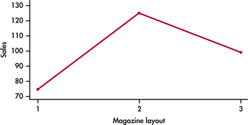
A magazine publisher wants to compare three different layouts for a magazine that will be displayed at supermarket checkout lines. She is interested in whether there is a layout that better impresses shoppers and results in more sales. To investigate, she randomly assigns 20 stores to each of the three layouts and records the number of magazines that are sold in a one-week period.
EXAMPLE 14.2 Average Age of Customers?

How do five Starbucks coffeehouses in the same city differ in the demographics of their customers? Are certain coffeehouses more popular among millennials? A market researcher asks 50 customers of each store to respond to a questionnaire. One variable of interest is the customer’s age.
These two examples are similar in that
- There is a single quantitative response variable measured on many units; the units are the stores in the first example and customers in the second.Page 713
- The goal is to compare several populations: stores displaying three magazine layouts in the first example and customers of the five coffeehouses in the second.
- There is a single categorical explanatory variable, or factor, that classifies these populations: magazine layout in the first example and coffeehouse in the second.
experiment
observational study
There is, however, an important difference. Example 14.1 describes an experiment in which stores are randomly assigned to layouts. Example 14.2 is an observational study in which customers are selected during a particular time of day and not all agree to provide data. We treat our samples of customers as random samples even though this is only approximately true.
In both examples, we use ANOVA to compare the mean responses. The response variable is the number of magazines sold in the first example and the age of the customer in the second. The same ANOVA methods apply to data from randomized experiments and to data from random samples. Do keep the method by which data are produced in mind when interpreting the results, however. A strong case for causation is best made by a randomized experiment.
Comparing means
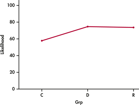
The question we ask in ANOVA is, “Do all groups have the same population mean?” We often use the term groups for the populations to be compared in a one-way ANOVA. To answer this question, we compare sample means. Figure 14.1 displays the sample means for Example 14.1. Layout 2 has the highest average sales. But are the observed differences among the sample means just the result of chance variation? We do not expect sample means to be equal even if the population means are all identical.
The purpose of ANOVA is to assess whether the observed differences among sample means are statistically significant. In other words, could variation in sample means this large be plausibly due to chance, or is it good evidence for a difference among the population means? This question can’t be answered from the sample means alone. Because the standard deviation of a sample mean ˉx is the population standard deviation σ divided by √n, the answer depends upon both the variation within the groups of observations and the sizes of the samples.
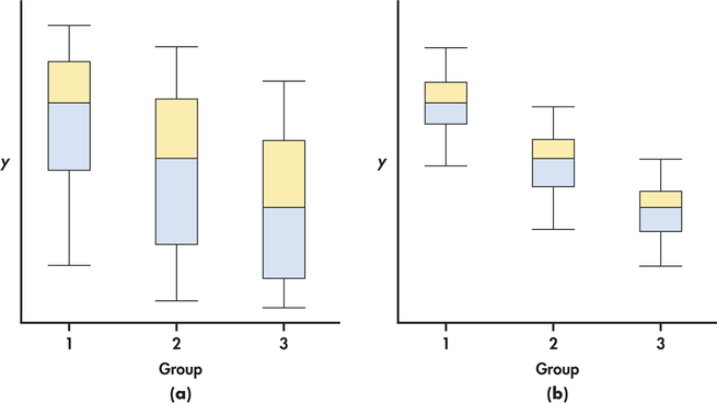
Side-by-side boxplots help us see the within-group variation. Compare Figures 14.2(a) and 14.2(b). The sample medians are the same in both figures, but the large variation within the groups in Figure 14.2(a) suggests that the differences among sample medians could be due simply to chance. The data in Figure 14.2(b) are much more convincing evidence that the populations differ.
Even the boxplots omit essential information, however. To assess the observed differences, we must also know how large the samples are. Nonetheless, boxplots are a good preliminary display of ANOVA data. While ANOVA compares means and boxplots display medians, these two measures of center will be close together for distributions that are nearly symmetric. If the distributions are not symmetric, we may consider a transformation prior to displaying and analyzing the data.
The two-sample t statistic
Two-sample t statistics compare the means of two populations. If the two populations are assumed to have equal but unknown standard deviations and the sample sizes are both equal to n, the t statistic is
t=ˉx1−ˉx2sp√1n+1n=√n2(ˉx1−ˉx2)sp
The square of this t statistic is
t2=n2(ˉx1−ˉx2)2s2p
If we use ANOVA to compare two populations, the ANOVA F statistic is exactly equal to this t2. Thus, we can learn something about how ANOVA works by looking carefully at the statistic in this form.
between-group variation
The numerator in the t2 statistic measures the variation between the groups in terms of the difference between their sample means ˉx1 and ˉx2. This is multiplied by a factor for the common sample size n. The numerator can be large because of a large difference between the sample means or because the common sample size n is large.
within-group variation
The denominator measures the variation within groups by s2p, the pooled estimator of the common variance. If the within-group variation is small, the same variation between the groups produces a larger statistic and, thus, a more significant result.
Although the general form of the F statistic is more complicated, the idea is the same. To assess whether several populations all have the same mean, we compare the variation among the means of several groups with the variation within groups. Because we are comparing variation, the method is called analysis of variance.
An overview of ANOVA
ANOVA tests the null hypothesis that the population means are all equal. The alternative is that they are not all equal. This alternative could be true because all of the means are different or simply because one of them differs from the rest. Because this alternative is a more complex situation than comparing just two populations, we need to perform some further analysis if we reject the null hypothesis. This additional analysis allows us to draw conclusions about which population means differ from others and by how much.
The computations needed for ANOVA are more lengthy than those for the t test. For this reason, we generally use computer software to perform the calculations. Automating the calculations frees us from the burden of arithmetic and allows us to concentrate on interpretation.


moral
It seems as if every day we hear of another public figure acting badly. In business, immoral actions by a CEO not only threaten the CEO’s professional reputation, but can also affect his or her company’s bottom line. Quite often, however, consumers continue to support the company regardless of how they feel about the actions. A group of researchers propose this is because consumers engage in moral decoupling.1 This is a process by which judgments of performance are separated from judgments of morality.
To demonstrate this, the researchers performed an experiment involving 121 participants. Each participant was randomly assigned to one of three groups: moral decoupling, moral rationalization, or a control. For the first two groups, participants were primed by reading statements either arguing that immoral actions should remain separate from judgments of performance (moral decoupling) or statements arguing that people should not always be at fault for their immoral actions because of situational pressures (moral rationalization). In the control group, participants read about the importance of humor.
All participants then read a scenario about a CEO of a consumer electronics company who had helped his company become a leader in innovative and stylish products over the course of the past decade. Last month, however, he was caught in a scandal and confirmed he supported racist and sexist hiring policies. After reading the scenario, participants were asked to indicate their likelihood of purchasing the company’s products in the future by answering several items, measured on a 0–100 scale. They were also asked to judge the CEO’s degree of immorality by answering a couple of items measured on a 0–7 scale. Let’s focus on the likelihood of purchase and leave the immorality judgment analysis as a later exercise. Here is a summary of the data:
| Group | n | ˉx | s |
| Control | 41 | 58.11 | 22.88 |
| Moral decoupling | 43 | 75.06 | 16.35 |
| Moral rationalization | 37 | 74.04 | 18.02 |
The two moral reasoning groups have higher sample means than the control group, suggesting people in these two groups are more likely to buy this company’s products in the future. ANOVA will allow us to determine whether this observed pattern in sample means can be extended to the group means.

We should always start an ANOVA with a careful examination of the data using graphical and numerical summaries in order to get an idea of what to expect from the analysis and also to check for unusual patterns in the data. Just as in linear regression and the two-sample t methods, outliers and extreme departures from Normality can invalidate the computed results.
EXAMPLE 14.3 A Graphical Summary of the Data
moral
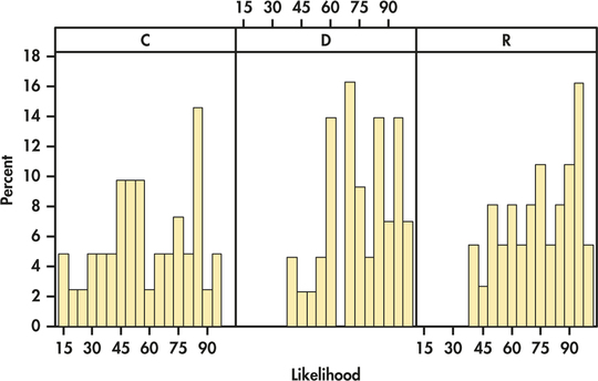
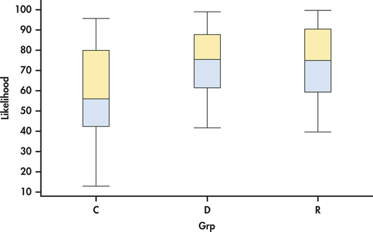
CASE 14.1 Histograms of the three groups are given in Figure 14.3. Note that the heights of the bars are percents rather than counts. This is commonly done when the group sizes vary. Figure 14.4 gives side-by-side boxplots for these data. We see that the likelihood scores cover most of the range of possible values. We also see a lot of overlap in the scores across groups. There do not appear to be any outliers, and the histograms show some, but not severe, skewness.
The three sample means are plotted in Figure 14.5. The control group mean appears to be lower than the other two. However, given the large amount of overlap in the data across groups, this pattern could just be the result of chance variation. We use ANOVA to make this determination.
In the setting of Case 14.1, we have an experiment in which participants were randomly assigned to one of three groups. Each of these groups has a mean, and our inference asks questions about these means. The participants in this study were all recruited through the same university. They also participated in return for financial payment.
Formulating a clear definition of the populations being compared with ANOVA can be difficult. Often, some expert judgment is required, and different consumers of the results may have differing opinions. Whether the samples in this study should be considered as SRSs from the population of consumers at the university or from the population of all consumers in the United States is open for debate. Regardless, we are more confident in generalizing our conclusions to similar populations when the results are clearly significant than when the level of significance just barely passes the standard of P=0.05.
We first ask whether or not there is sufficient evidence in the data to conclude that the corresponding population means are not all equal. Our null hypothesis here states that the population mean score is the same for all three groups. The alternative is that they are not all the same. Rejecting the null hypothesis that the means are all the same using ANOVA is not the same as concluding that all the means are different from one another. The ANOVA null hypothesis can be false in many different ways. Additional analysis is required to compare the three means.
contrasts
The researchers hypothesize that these moral reasoning strategies should allow a consumer to continue to support the company. Therefore, a reasonable question to ask is whether or not the mean for the control group is smaller than the others. When there are particular versions of the alternative hypothesis that are of interest, we use contrasts to examine them. Note that, to use contrasts, it is necessary that the questions of interest be formulated before examining the data. It is cheating to make up these questions after analyzing the data.
multiple comparisons
If we have no specific relations among the means in mind before looking at the data, we instead use a multiple-comparisons procedure to determine which pairs of population means differ significantly. In the next section, we explore both contrasts and multiple comparisons in detail.
Apply Your Knowledge
Question 14.1
14.1 What’s wrong?
For each of the following, explain what is wrong and why.
- ANOVA tests the null hypothesis that the sample means are all equal.
- Within-group variation is the variation in the data due to the differences in the sample means.
- You use one-way ANOVA to compare the variances of several populations.
- A multiple-comparisons procedure is used to compare a relation among means that was specified prior to looking at the data.
14.1
(a) ANOVA does not test the sample means; it should be the population means. (b) This is not within-group variation, it is between-group variation. (c) We are not comparing the variances, we are comparing the means of several populations. (d) This is true for contrasts, not multiplecomparisons. Multiple-comparisons are used when we have no specific relations among means in mind before looking at the data.
Question 14.2
14.2 What’s wrong?
For each of the following, explain what is wrong and why.
- In rejecting the null hypothesis, we conclude that all the means are different from one another.
- The ANOVA F statistic will be large when the within-group variation is much larger than the between-group variation.
- A two-way ANOVA is used when comparing two populations.
- A strong case for causation is best made by an observational study.
The ANOVA model
When analyzing data, the following equation reminds us that we look for an overall pattern and deviations from it:
DATA=FIT+RESIDUAL
In the regression model of Chapter 10, the FIT was the population regression line, and the RESIDUAL represented the deviations of the data from this line. We now apply this framework to describe the statistical models used in ANOVA. These models provide a convenient way to summarize the conditions that are the foundation for our analysis. They also give us the necessary notation to describe the calculations needed.
First, recall the statistical model for a random sample of observations from a single Normal population with mean μ and standard deviation σ. If the observations are
x1, x2, …, xn
we can describe this model by saying that the xj are an SRS from the N(μ, σ) distribution. Another way to describe the same model is to think of the x’s varying about their population mean. To do this, write each observation xj as
xj=μ+∈j
The ∈j are then an SRS from the N(0, σ) distribution. Because μ is unknown, the ∈’s cannot actually be observed. This form more closely corresponds to our
DATA=FIT+RESIDUAL
way of thinking. The FIT part of the model is represented by μ. It is the systematic part of the model. The RESIDUAL part is represented by ∈j. It represents the deviations of the data from the fit and is due to random, or chance, variation.
There are two unknown parameters in this statistical model: μ and σ. We estimate μ by ˉx, the sample mean, and σ by s, the sample standard deviation. The differences ej=xj−ˉx are the residuals and correspond to the ∈j in this statistical model.
The model for one-way ANOVA is very similar. We take random samples from each of I different populations. The sample size is ni for the ith population. Let xij represent the jth observation from the ith population. The I population means are the FIT part of the model and are represented by μi. The random variation, or RESIDUAL, part of the model is represented by the deviations ∈ij of the observations from the means.
The One-Way ANOVA Model
The data for one-way ANOVA are SRSs from each of I populations. The sample from the ith population has ni observations, xi1, xi2, …, xini. The one-way ANOVA model is
xij=μi+∈ij
for i=1, …, I and j=1, …, ni. The ∈ij are assumed to be from an N(0, σ) distribution. The parameters of the model are the I population means μ1, μ2, …, μI and the common standard deviation σ.
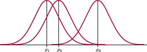
Note that the sample sizes ni may differ, but the standard deviation σ is assumed to be the same in all the populations. Figure 14.6 pictures this model for I=3. The three population means μi are all different, but the spreads of the three Normal distributions are the same, reflecting the condition that all three populations have the same standard deviation.
EXAMPLE 14.4 ANOVA Model for the Moral Reasoning Study
CASE 14.1 In Case 14.1, there are three groups that we want to compare, so I=3. The population means μ1, μ2, and μ3 are the mean values for the control group, moral decoupling group, and moral rationalization group, respectively. The sample sizes ni are 41, 43, and 37, respectively. It is common to use numerical subscripts to distinguish the different means, and some software requires that levels of factors in ANOVA be specified as numerical values. An alternative is to use subscripts that suggest the actual groups. In our example, we could replace μ1, μ2, and μ3 by μC, μD, and μR, respectively.
The observation x11, for example, is the likelihood score for the first participant in the control group. Accordingly, the data for the other control group participants are denoted by x12, x13, and so on. Similarly, the data for the other two groups have a first subscript indicating the group and a second subscript indicating the participant in that group.
According to our model, the score for the first participant in the control group is x11=μ1+ ∈11, where μ1 is the average for the population of all consumers and ∈11 is the chance variation due to this particular participant. Similarly, the score for the last participant assigned to the moral rationalization group is x3,37=μ3+ ∈3,37, where μ3 is the average score for all consumers primed with moral rationalization and ∈3,37 is the chance variation due to this participant.
The ANOVA model assumes that the deviations ∈ij are independent and Normally distributed with mean 0 and standard deviation σ. For Case 14.1, we have clear evidence that the data are not Normal. The values are numbers that can only range from 0 to 100, and we saw some skewness in the group distributions (Figure 14.3, page 716). However, because our inference is based on the sample means, which will be approximately Normal given the sample sizes, we are not overly concerned about this violation of model assumptions.
Apply Your Knowledge
Question 14.3
14.3 Magazine layouts.
Example 14.1 (page 712) describes a study designed to compare sales based on different magazine layouts. Write out the ANOVA model for this study. Be sure to give specific values for I and the ni. List all the parameters of the model.
14.3
xij=μi+εij, i=1, 2, 3, j=1, 2, … , ni. εij~N(0, σ). The parameters of the model are μ1, μ2, μ3, and σ.
Question 14.4
14.4 Ages of customers at different coffeehouses.
In Example 14.2 (page 712), the ages of customers at different coffeehouses are compared. Write out the ANOVA model for this study. Be sure to give specific values for I and the ni. List all the parameters of the model.
Estimates of population parameters
The unknown parameters in the statistical model for ANOVA are the I population means μi and the common population standard deviation σ. To estimate μi we use the sample mean for the ith group:
ˉxi=1nini∑j=1xij
residuals
The residuals eij=xij−ˉxi reflect the variation about the sample means that we see in the data and are used in the calculations of the sample standard deviations
si=√∑nij=1(xij−ˉxi)2ni−1
In addition to the deviations being Normally distributed, the ANOVA model also states that the population standard deviations are all equal. Before estimating σ, it is important to check this equality assumption using the sample standard deviations. Most computer software provides at least one test for the equality of standard deviations. Unfortunately, many of these tests lack robustness against non-Normality.
Because ANOVA procedures are not extremely sensitive to unequal standard deviations, we do not recommend a formal test of equality of standard deviations as a preliminary to the ANOVA. Instead, we use the following rule of thumb.
Rule for Examining Standard Deviations in ANOVA
If the largest sample standard deviation is less than twice the smallest sample standard deviation, we can use methods based on the condition that the population standard deviations are equal and our results will still be approximately correct.2
If there is evidence of unequal population standard deviations, we generally try to transform the data so that they are approximately equal. We might, for example, work with √xij or log xij. Fortunately, we can often find a transformation that both makes the group standard deviations more nearly equal and also makes the distributions of observations in each group more nearly Normal (see Exercises 14.65 and 14.66 later in the chapter). If the standard deviations are markedly different and cannot be made similar by a transformation, inference requires different methods that are beyond the scope of this book.
EXAMPLE 14.5 Are the Standard Deviations Equal?
moral
CASE 14.1 In the moral reasoning study, there are I=3 groups and the sample standard deviations are s1=22.88, s2=16.35, and s3=18.02. The largest standard deviation (22.88) is not larger than twice the smallest (2×16.35=32.70), so our rule of thumb indicates we can assume the population standard deviations are equal.
When we assume that the population standard deviations are equal, each sample standard deviation is an estimate of σ. To combine these into a single estimate, we use a generalization of the pooling method introduced in Chapter 7 (page 387).
Pooled Estimator of σ
Suppose we have sample variances s21, s22, …, s2I from I independent SRSs of sizes n1, n2, …, nI from populations with common variance σ2. The pooled sample variance
s2p=(n1−1)s21+(n2−1)s22+⋯+(nI−1)s2I(n1−1)+(n2−1)+⋯+(nI−1)
is an unbiased estimator of σ2. The pooled standard error
sp=√s2p
is the estimate of σ.
Pooling gives more weight to groups with larger sample sizes. If the sample sizes are equal, s2p is just the average of the I sample variances. Note that sp is not the average of the I sample standard deviations.
EXAMPLE 14.6 The Common Standard Deviation Estimate
moral
CASE 14.1 In the moral reasoning study, there are I=3 groups and the sample sizes are n1=41, n2=43, and n3=37. The sample standard deviations are s1=22.88, s2=16.35, and s3=18.02, respectively.
The pooled variance estimate is
s2p=(n1−1)s21+(n2−1)s22+(n3−1)s23(n1−1)+(n2−1)+(n3−1)=(40)(22.88)2+(42)(16.35)2+(36)(18.02)2 40+42+36=43,857.26118=371.67
The pooled standard deviation is
sp=√371.67=19.28
This is our estimate of the common standard deviation σ of the likelihood scores in the three populations of consumers.
Apply Your Knowledge
Question 14.5
14.5 Magazine layouts.
Example 14.1 (page 712) describes a study designed to compare sales based on different magazine layouts, and in Exercise 14.3 (page 720), you described the ANOVA model for this study. The three layouts are designated 1, 2, and 3. The following table summarizes the sales data.
| Layout | ˉx | s | n |
| 1 | 75 | 55 | 20 |
| 2 | 125 | 63 | 20 |
| 3 | 100 | 58 | 20 |
- Is it reasonable to pool the standard deviations for these data? Explain your answer.
- For each parameter in your model from Exercise 14.3, give the estimate.
14.5
(a) Yes, the largest s is less than twice the smallest s, 63<2(55)=110. (b) The estimates for μ1, μ2, and μ3 are 75, 125, and 100. The estimate for σ3 is 58.7594.
Question 14.6
14.6 Ages of customers at different coffeehouses.
In Example 14.2 (page 712) the ages of customers at different coffeehouses are compared, and you described the ANOVA model for this study in Exercise 14.4 (page 720). Here is a summary of the ages of the customers:
| Store | ˉx | s | n |
| A | 38 | 8 | 50 |
| B | 44 | 10 | 50 |
| C | 43 | 11 | 50 |
| D | 35 | 7 | 50 |
| E | 40 | 9 | 50 |
- Is it reasonable to pool the standard deviations for these data? Explain your answer.
- For each parameter in your model from Exercise 14.4, give the estimate.
Testing hypotheses in one-way ANOVA
Comparison of several means is accomplished by using an F statistic to compare the variation among groups with the variation within groups. We now show how the F statistic expresses this comparison. Calculations are organized in an ANOVA table, which contains numerical measures of the variation among groups and within groups.
Reminder

ANOVA table, p.524
First, we must specify our hypotheses for one-way ANOVA. As usual, I represents the number of populations to be compared.
Hypotheses for One-Way ANOVA
The null and alternative hypotheses for one-way ANOVA are
H0:μ1=μ2=⋯=μIHa:not all of the μi are equal
We now use the moral strategy study (Case 14.1, page 715) to illustrate how to do a one-way ANOVA. Because the calculations are generally performed using statistical software on a computer, we focus on interpretation of the output.
EXAMPLE 14.7 Verifying the Conditions for ANOVA
moral
CASE 14.1 If ANOVA is to be trusted, three conditions must hold. Here is a summary of those conditions and our assessment of the data for Case 14.1.
SRSs. Can we regard the three groups as SRSs from three populations? An ideal study would start with an SRS from the population of interest and then randomly assign each participant to one of the groups. This usually isn’t practical. The researchers randomly assigned participants recruited from one university and paid them to participate. Can we act as if these participants were randomly chosen from the university or from the population of all consumers? People may disagree on the answer.
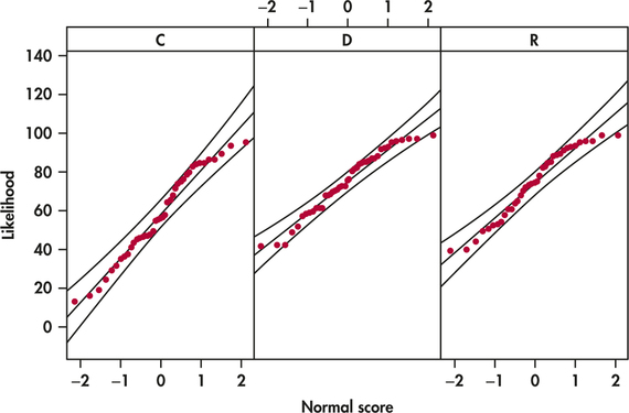
Normality. Are the likelihood scores Normally distributed in each group? Figure 14.7 displays Normal quantile plots for the three groups. The data look approximately Normal. Because inference is based on the sample means and we have relatively large sample sizes, we do not need to be concerned about violating this assumption.
Common standard deviation. Are the population standard deviations equal? Because the largest sample standard deviation is not more than twice the smallest sample standard deviation, we can proceed assuming the population standard deviations are equal.
Because we feel our data satisfy these three conditions, we proceed with the analysis of variance.
EXAMPLE 14.8 Are the Differences Significant?
moral
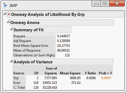
CASE 14.1 The ANOVA results produced by JMP are shown in Figure 14.8. The pooled standard deviation sp is reported as 19.28. The calculated value of the F statistic appears under the heading “F Ratio,” and its P-value is under the heading “Prob > F.” The value of F is 9.927, with a P-value of 0.0001. That is, an F of 9.927 or larger would occur by chance one time in 10,000 when the population means are equal. We can reject the null hypothesis that the three populations have equal means for any common choice of significance level. There is very strong evidence that the three populations of consumers do not all have the same mean score.
This concludes the basics of ANOVA: we first state the hypotheses, then verify that the conditions for ANOVA are met (Example 14.7), and finally look at the F statistic and its P-value, and state a conclusion (Example 14.8).
Apply Your Knowledge
Question 14.7
CASE 14.114.7 An alternative Normality check.
Figure 14.7 displays separate Normal quantile plots for the three groups. An alternative procedure is to make one Normal quantile plot using the eij=xij−ˉxi for all three groups together. Make this plot and summarize what it shows.
14.7
The data have constant variance. The Normal quantile plot shows the residuals are Normally distributed.
moral
The ANOVA table
Software ANOVA output contains more than simply the test statistic. The additional information shows, among other things, where the test statistic comes from.
The information in an analysis of variance is organized in an ANOVA table. In the software output in Figure 14.8, the columns of this table are labeled “Source,” “DF,” “Sum of Squares,” “Mean Square,” “F Ratio,” and “Prob > F” The rows are labeled “Grp,” “Error,” and “C. Total.” These are the three sources of variation in the one-way ANOVA. “Grp” was the name used in entering the data to distinguish the three treatment groups. Other software may use different column and row names but the rest of the table will be similar.
The Grp row in the table corresponds to the FIT term in our DATA = FIT + RESIDUAL way of thinking. It gives information related to the variation among group means. The ANOVA model allows the groups to have different means.
variation among groups
The Error row in the table corresponds to the RESIDUAL term in DATA = FIT + RESIDUAL. It gives information related to the variation within groups. The term error is most appropriate for experiments in the physical sciences, where the observations within a group differ because of measurement error. In business and the biological and social sciences, on the other hand, the within-group variation is often due to the fact that not all firms or plants or people are the same. This sort of variation is not due to errors and is better described as residual.
variation within groups
Finally, the Total row in the table corresponds to the DATA term in our DATA = FIT + RESIDUAL framework. So, for analysis of variance,
DATA = FIT + RESIDUAL
translates into
total variation = variation among groups + variation within groups
The ANOVA idea is to break the total variation in the responses into two parts: the variation due to differences among the group means and that due to differences within groups. Variation is expressed by sums of squares. We use SSG, SSE, and SST for the sums of squares for groups, error, and total, respectively. Each sum of squares is the sum of the squares of a set of deviations that expresses a source of variation. SST is the sum of squares of xij−ˉx, which measure variation of the responses around their overall mean. Variation of the group means around the overall mean ˉxi−ˉx is measured by SSG. Finally, SSE is the sum of squares of the deviations xij−ˉxi of each observation from its group mean.
Reminder
sum of squares, p.521
EXAMPLE 14.9 Sums of Squares for the Three Sources of Variation
CASE 14.1 The SS column in Figure 14.8 gives the values for the three sums of squares. They are
SSG=7377.895SSE=43,851.523SSE=51,229.418
In this example it appears that most of the variation is coming from Error, that is, from within groups. Verify that SST = SSG + SSE.
It is always true that SST = SSG + SSE. This is the algebraic version of the ANOVA idea: total variation is the sum of between-group variation and within-group variation.
Associated with each sum of squares is a quantity called the degrees of freedom Because SST measures the variation of all N observations around the overall mean, its degrees of freedom are DFT=N−1 , the degrees of freedom for the sample variance of the N responses. Similarly, because SSG measures the variation of the I sample means around the overall mean, its degrees of freedom are DFT=I−1. Finally, SSE is the sum of squares of the deviations xij−ˉxi. Here, we have N observations being compared with I sample means and DFE=N−1.
EXAMPLE 14.10 Degrees of Freedom for the Three Sources
CASE 14.1 In Case 14.1, we have I=3 and N=121. Therefore,
DFG=I−1=3−1=2DFE=N−1=121−3=118DFT=N−1=121−1=120
These are the entries in the DF column in Figure 14.8.
Note that the degrees of freedom add in the same way that the sums of squares add. That is, DFT=DFG+DFE.
For each source of variation, the mean square is the sum of squares divided by the degrees of freedom. You can verify this by doing the divisions for the values given on the output in Figure 14.8. Generally, the ANOVA table includes mean squares only for the first two sources of variation. The mean square corresponding to the total source is the sample variance that we would calculate assuming that we have one sample from a single population—that is, assuming that the means of the three groups are the same.
Reminder
mean square, p.522
Sums of Squares, Degrees of Freedom, and Mean Squares
Sums of squares represent variation present in the data. They are calculated by summing squared deviations. In one-way ANOVA, there are three sources of variation: groups, error, and total. The sums of squares are related by the formula
SST=SSG+SSE
Thus, the total variation is composed of two parts, one due to groups and one due to “error” (variation within groups).
Degrees of freedom are related to the deviations that are used in the sums of squares. The degrees of freedom are related in the same way as the sums of squares:
DFT=DFG+DFE
To calculate each mean square, divide the corresponding sum of squares by its degrees of freedom.
We can use the mean square for error to find sp, the pooled estimate of the parameter σ of our model. It is true in general that
s2p=MSE=SSEDFE
In other words, the mean square for error is an estimate of the within-group variance, σ2. The estimate of σ is therefore the square root of this quantity. So,
sp=√MSE
Apply Your Knowledge
Question 14.8
14.8 Computing the pooled variance estimate.
In Example 14.6 (page 721), we computed the pooled standard deviation sp using the population standard deviations and sample sizes. Now use the MSE from the ANOVA table in Figure 14.8 to estimate σ. Verify that it is the same value.
Question 14.9
CASE 14.114.9 Total mean square.
The output does not give the total mean square MST = SST/DFT. Calculate this quantity. Then find the mean and variance of all 121 observations and verify that MST is the variance of all the responses.
14.9
MST=426.9118. The mean is 69.0052; the variance is 426.9118.
moral
The F test
If H0 is true, there are no differences among the group means. In that case, MSG will reflect only chance variation and should be about the same as MSE. The ANOVA F statistic simply compares these two mean squares, F=MSG/MSE. Thus, this statistic is near 1 if H0 is true and tends to be larger if Ha is true. In our example, MSG=3688.95 and MSE=371.62, so the ANOVA F statistic is
F=MSGMSE=3688.95371.62=9.93
When H0 is true, the F statistic has an F distribution that depends on two numbers: the degrees of freedom for the numerator and the degrees of freedom for the denominator. These degrees of freedom are those associated with the mean squares in the numerator and denominator of the F statistic. For one-way ANOVA, the degrees of freedom for the numerator are DFG=I−1 and the degrees of freedom for the denominator are DFE=N−1. We use the notation F(I−1,N−I) for this distribution.

The One-Way ANOVA applet is an excellent way to see how the value of the F statistic and its P-value depend on both the variability of the data within the groups and the differences between the group means. Exercises 14.12 and 14.13 (page 729) make use of this applet.
The ANOVA F test shares the robustness of the two-sample t test. It is relatively insensitive to moderate non-Normality and unequal variances, especially when the sample sizes are similar. The constant variance assumption is more important when we compare means using contrasts and multiple comparisons, additional analyses that are generally performed after the ANOVA F test. We discuss these analyses in the next section.
The ANOVA F test
To test the null hypothesis in a one-way ANOVA, calculate the F statistic
|
F=MSGMSE |
 |
When H0 is true, the F statistic has the F(I−1,N−I) distribution. When Ha is true, the F statistic tends to be large. We reject H0 in favor of Ha if the F statistic is sufficiently large.
The P-value of the F test is the probability that a random variable having the F(I−1,N−I) distribution is greater than or equal to the calculated value of the F statistic.
Tables of F critical values are available for use when software does not give the P-value. Table E in the back of the book contains the F critical values for probabilities p=0.100,0.050,0.025,0.010, and 0.001. For one-way ANOVA, we use critical values from the table corresponding to I−1 degrees of freedom in the numerator and N−I degrees of freedom in the denominator. When determining the P-value, remember that the F test is always one-sided because any differences among the group means tend to make F large.
EXAMPLE 14.11 Comparing the Likelihood of Purchase Scores
CASE 14.1 In the moral strategy study, F=9.93. There are three populations, so the degrees of freedom in the numerator are DFG=I−1=2. The degrees of freedom in the denominator are DFE=N−1=121−3=118. In Table E, first find the column corresponding to two degrees of freedom in the numerator. For the degrees of freedom in the denominator, there are entries for 100 and 200. These entries are very close. To be conservative, we use critical values corresponding to 100 degrees of freedom in the denominator because these are slightly larger. Because 9.93 is beyond 7.41, we reject H0 and conclude that the differences in means are statistically significant, with P<0.001.
| p | Critical value |
| 0.100 | 2.36 |
| 0.050 | 3.09 |
| 0.025 | 3.83 |
| 0.010 | 4.82 |
| 0.001 | 7.41 |
The following display shows the general form of a one-way ANOVA table with the F statistic. The formulas in the sum of squares column can be used for calculations in small problems. There are other formulas that are more efficient for hand or calculator use, but ANOVA calculations are usually done by computer software.
| Source | Degrees of freedom |
Sum of squares | Means square |
F |
| Groups | I−1 | ∑groupsni(ˉxi−ˉx)2 | SSG/DFG | MSG/MSE |
| Error | N−I | ∑groups(ni−1)s2i | SSE/DFE | |
| Total | N−1 | ∑obs(xij−ˉx)2 | SST/DFT |
One other item given by some software for ANOVA is worth noting. For an analysis of variance, we define the coefficient of determination as
R2=SSGSST
coefficient of
determination
The coefficient of determination plays the same role as the squared multiple correlation R2 in a multiple regression. We can easily calculate the value from the ANOVA table entries.
EXAMPLE 14.12 Coefficient of Determination for Moral Strategy Study
The software-generated ANOVA table for Case 14.1 is given in Figure 14.8 (page 724). From that display, we see that SSG=7377.895 and SST=51,229.418. The coefficient of determination is
R2=SSGSST=7377.89551,229.418=0.14
About 14% of the variation in the likelihood scores is explained by the different groups. The other 86% of the variation is due to participant-to-participant variation within each of the groups. We can see this in the histograms of Figure 14.3 (page 716) and the boxplots of Figure 14.4 (page 716). Each of the groups has a large amount of variation, and there is a substantial amount of overlap in the distributions. The fact that we have strong evidence (P<0.001) against the null hypothesis that the three population means are all the same does not tell us that the distributions of values are far apart.
Apply Your Knowledge
Question 14.10
14.10 What’s wrong?
For each of the following, explain what is wrong and why.
- The pooled estimate sp is a parameter of the ANOVA model.
- The mean squares in an ANOVA table will add, that is, MST=MSG+MSE.
- For an ANOVA F test with P=0.31, we conclude that the means are the same.
- A very small F test P-value implies that the group distributions of responses are far apart.
Question 14.11
14.11 Use Table E.
An ANOVA is run to compare four groups. There are eight subjects in each group.
- Give the degrees of freedom for the ANOVA F statistic.
- How large would this statistic need to be to have a P-value less than 0.05?
- Suppose that we are still interested in comparing the four groups, but we obtain data on 16 subjects per group. How large would the F statistic need to be to have a P-value less than 0.05?
- Explain why the answer to part (c) is smaller than what you found for part (b).
14.11
(a) DFG=I−1=4−1=3. DFE=N−I=32−4=28. (b) Bigger than 2.95. (c) Bigger than 2.76. (d) More observations per group gives a larger DFE, which makes the F critical value smaller. Conceptually, more data give more information showing the group differences and giving more evidence the differences we are observing are real and not due to chance. Thus, a larger DFE will give a smaller critical value and smaller P-value.
Question 14.12
14.12 The effect of within-group variation.
Go to the One-Way ANOVA applet. In the applet display, the black dots are the mean responses in three treatment groups. Move these up and down until you get a configuration with P-value about 0.01. Note the value of the F statistic. Now increase the variation within the groups without changing their means by dragging the mark on the standard deviation scale to the right. Describe what happens to the F statistic and the P-value. Explain why this happens.
Question 14.13
14.13 The effect of between-group variation.
Go to the One-Way ANOVA applet. Set the standard deviation near the middle of its scale and drag the black dots so that the three group means are approximately equal. Note the value of the F statistic and its P-value. Now increase the variation among the group means: drag the mean of the second group up and the mean of the third group down. Describe the effect on the F statistic and its P-value. Explain why they change in this way.
14.13
More variation between the groups makes the F statistic larger and the P-value smaller. This happens because the more variation we have between groups suggests that the differences we are seeing are actually due to actual differences between the groups, not just chance, giving us more evidence of group differences.
Using software
We have used JMP to illustrate the analysis of the moral strategy study data. Other statistical software gives similar output, and you should be able to extract all the ANOVA information we have discussed. Here is an example on which to practice this skill.
EXAMPLE 14.13 Do Eyes Affect Ad Response?
eyes
Research from a variety of fields has found significant effects of eye gaze and eye color on emotions and perceptions such as arousal, attractiveness, and honesty. These findings suggest that a model’s eyes may play a role in a viewer’s response to an ad.
In one study, students in marketing and management classes of a southern, predominantly Hispanic, university were each presented with one of four portfolios.3 Each portfolio contained a target ad for a fictional product, Sparkle Toothpaste. Students were asked to view the ad and then respond to questions concerning their attitudes and emotions about the ad and product. All questions were from advertising-effects questionnaires previously used in the literature. Each response was on a 7-point scale.
Although the researchers investigated nine attitudes and emotions, we focus on the viewer’s “attitudes toward the brand.” This response was obtained by averaging 10 survey questions. The higher the score, the more favorable the attitude.
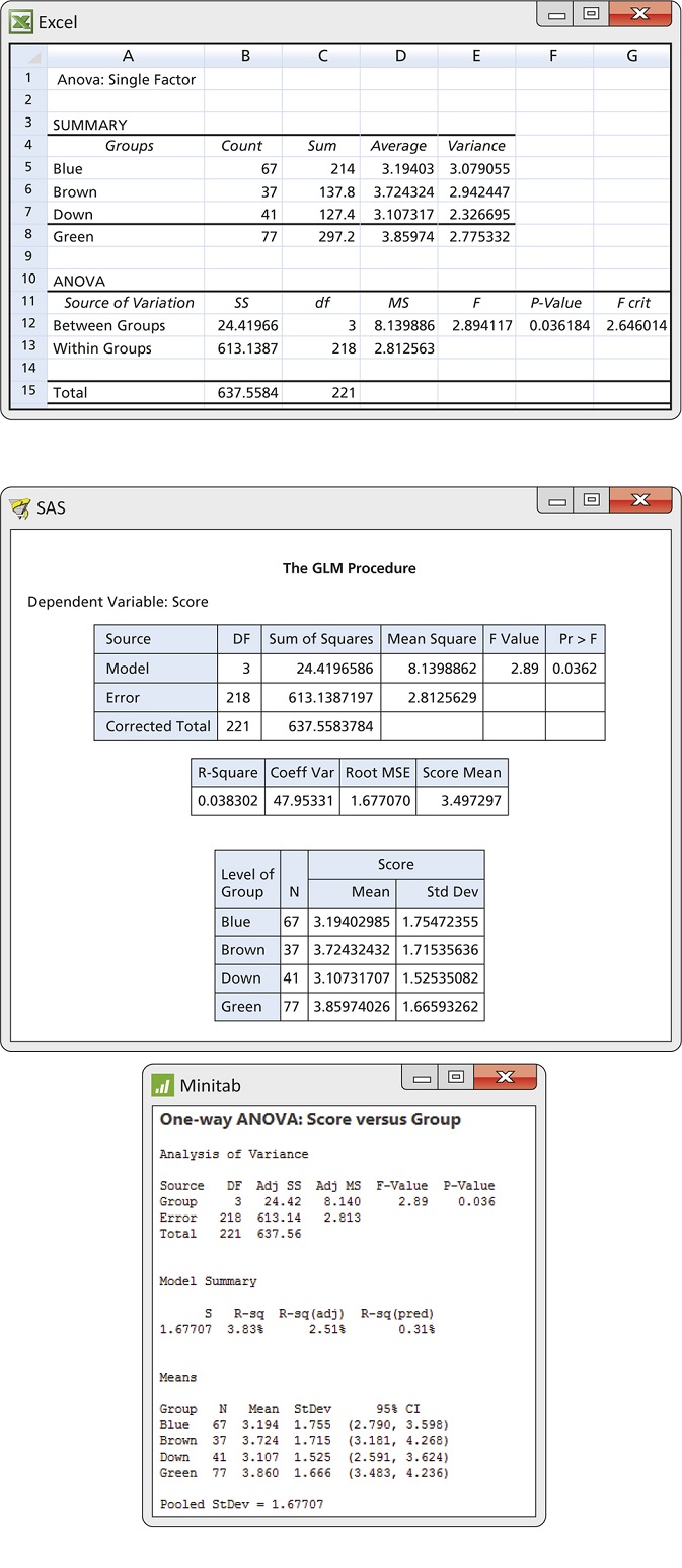
The target ads were created using two digital photographs of a model. In onepicture, the model is looking directly at the camera so the eyes can be seen. This picture was used in three target ads. The only difference was the model’s eyes, which were made to be either brown, blue, or green. In the second picture, the model is in virtually the same pose but looking downward so the eyes are not visible. A total of 222 surveys were used for analysis. The following table summarizes the responses for the four portfolios. Outputs from Excel, SAS, and Minitab are given in Figure 14.9.
| Group | n | ˉx | s |
| Blue | 67 | 3.19 | 1.75 |
| Brown | 37 | 3.72 | 1.72 |
| Green | 77 | 3.86 | 1.67 |
| Down | 41 | 3.11 | 1.53 |
There is evidence at the 5% significance level to reject the null hypothesis that the four groups have equal means (P=0.036). In Exercises 14.69 and 14.71 (page 756), you are asked to perform further inference using contrasts.
Apply Your Knowledge
Question 14.14
14.14 Compare software.
Refer to the output in Figure 14.9. Different names are given to the sources of variation in the ANOVA tables.
- What are the names given to the source we call Groups?
- What are the names given to the source we call Error?
- What are the reported P-values for the ANOVA F test?
Question 14.15
14.15 Compare software.
The pooled standard error for the data in Example 14.13 is sp=1.677. Look at the software output in Figure 14.9.
- Explain to someone new to ANOVA why SAS labels this quantity as “Root MSE.”
- Excel does not report sp. How can you find its value from Excel output?
14.15
(a) sp can be found by taking the square root of the MSE. (b) Take the square root of the Within Groups MS.
BEYOND THE BASICS: Testing the Equality of Spread
The two most basic descriptive features of a distribution are its center and spread. We have described procedures for inference about population means for Normal populations and found that these procedures are often useful for non-Normal populations as well. It is natural to turn next to inference about spread.
While the standard deviation is a natural measure of spread for Normal distributions, it is not for distributions in general. In fact, because skewed distributions have unequally spread tails, no single numerical measure is adequate to describe the spread of a skewed distribution. Because of this, we recommend caution when testing equal standard deviations and interpreting the results.
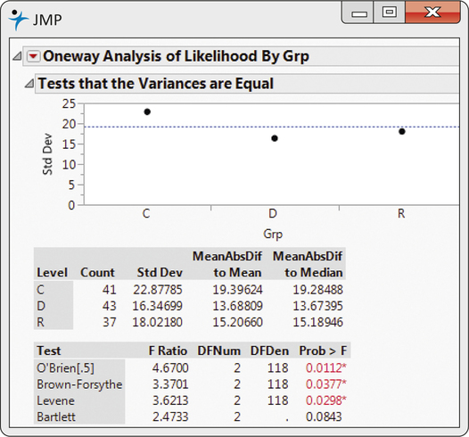
Most formal tests for equal standard deviations are extremely sensitive to non- Normal populations. Of the tests commonly available in software packages, we suggest using the modified Levene’s (or Brown-Forsythe) test due to its simplicity and robustness against non-Normal data.4 The test involves performing a one-way ANOVA on a transformation of the response variable, constructed to measure the spread in each group. If the populations have the same standard deviation, then the average deviation from the population center should also be the same.
Modified Levene’s Test for Equality of Standard Deviations
To test for the equality of the I population standard deviations, perform a onewayANOVA using the transformed response
yij=|xij−Mi|
where Mi is the sample median for population i. We reject the assumption of equal spread if the P-value of this test is less than the significance level α.
This test uses a more robust measure of deviation replacing the mean with the median and replacing squaring with the absolute value. Also, the transformed response variable is straightforward to create, so this test can easily be performed regardless of whether or not your software specifically has it.
EXAMPLE 14.14 Are the Standard Deviations Equal?
moral
CASE 14.1 Figure 14.10 shows output of the modified Levene’s test for the moral reasoning study. In both JMP and SAS, the test is called Brown-Forsythe. The P-value is 0.0377, which is smaller than α=0.05, suggesting the variances are not the same. This is not that surprising a result given the boxplots in Figure 14.4 (page 716). There, we see that the spread in the scores for the control group is much larger than the spread in the other two groups.
Remember that our rule of thumb (page 720) is used to assess whether different standard deviations will impact the ANOVA results. It’s not a formal test that the standard deviations are equal. In Exercises 14.65 and 14.66 (pages 755–756), we examine a transformation of the likelihood scores that better stabilizes the variances. Part of those exercises will be a comparison of the transformed likelihood score ANOVA results to the results of this section.