14.2 Comparing Group Means
 This page includes Video Technology Manuals
The ANOVA F test gives a general answer to a general question: are the differences among observed group means significant? Unfortunately, a small P-value simply tells us that the group means are not all the same. It does not tell us specifically which means differ from each other. Plotting and inspecting the means give us some indication of where the differences lie, but we would like to supplement inspection with formal inference. This section presents two approaches to the task of comparing group means.
Contrasts
The preferred approach is to pose specific questions regarding comparisons among the means before the data are collected. We can answer specific questions of this kind and attach a level of confidence to the answers we give. We now explore these ideas in the setting of Case 14.2.


eduprod

Your company markets educational materials aimed at parents of young children. You are planning a new product that is designed to improve children’s reading comprehension. Your product is based on new ideas from educational research, and you would like to claim that children will acquire better reading comprehension skills utilizing these new ideas than with the traditional approach. Your marketing material will include the results of a study conducted to compare two versions of the new approach with the traditional method.5 The standard method is called Basal, and the two variations of the new method are called DRTA and Strat.
Education researchers randomly divided 66 children into three groups of 22. Each group was taught by one of the three methods. The response variable is a measure of reading comprehension called COMP that was obtained by a test taken after the instruction was completed. Can you claim that the new methods are superior to Basal?
We can compare the new with the standard by posing and answering specific questions about the mean responses. First, here is the basic ANOVA.
EXAMPLE 14.15 Are the Comprehension Scores Different?
eduprod
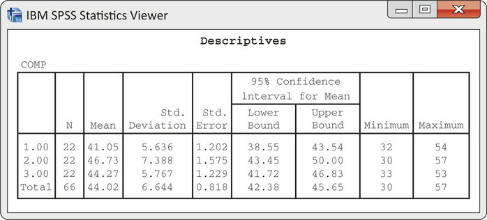
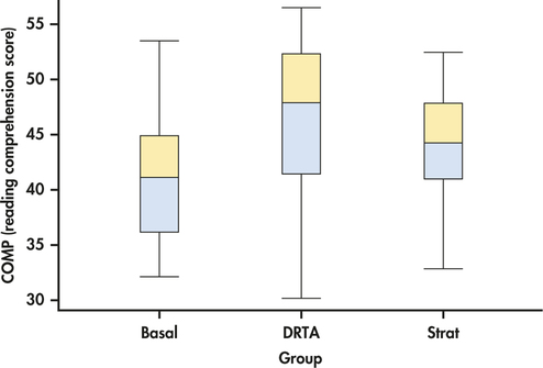
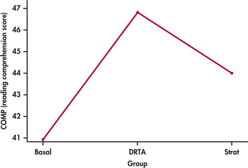
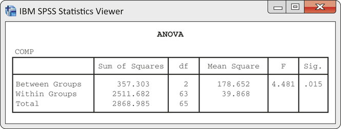
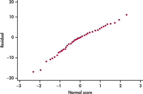
CASE 14.2 Figure 14.11 gives the summary statistics for COMP computed by SPSS. This software uses only numeric values for the factor, so we coded the groups as 1 for Basal, 2 for DRTA, and 3 for Strat. Side-by-side boxplots appear in Figure 14.12, and Figure 14.13 plots the group means. The ANOVA results generated by SPSS are given in Figure 14.14, and a Normal quantile plot of the residuals appears in Figure 14.15.
The ANOVA null hypothesis is
H0:μB=μD=μS
where the subscripts correspond to the group labels Basal, DRTA, and Strat. Figure 14.14 shows that F=4.48 with degrees of freedom 2 and 63. The P-value is 0.015. We have strong evidence against H0.
What can the researchers conclude from this analysis? The alternative hypothesis is true if μB≠μD or if μB≠μS or if μD≠μS or if any combination of these statements is true. We would like to be more specific.
EXAMPLE 14.16 The Major Question
CASE 14.2 The two new methods are based on the same idea. Are they superior to the standard method? We can formulate this question as the null hypothesis
H01:12(μD+μS)=μB
with the alternative
Ha1:12(μD+μS)>μB
The hypothesis H01 compares the average of the two innovative methods (DRTA and Strat) with the standard method (Basal). The alternative is one-sided because the researchers are interested in demonstrating that the new methods are better than the old. We use the subscripts 1 and 2 to distinguish two sets of hypotheses that correspond to two specific questions about the means.
EXAMPLE 14.17 A Secondary Question
CASE 14.2 A secondary question involves a comparison of the two new methods. We formulate this as the hypothesis that the methods DRTA and Strat are equally effective,
H02:μD=μS
versus the alternative
Ha2:μD≠μS
contrasts
Each of H01 and H02 says that a combination of population means is 0. These combinations of means are called contrasts. We use ψ the Greek letter psi, for contrasts among population means. The two contrasts that arise from our two null hypotheses are
ψ1=−μB+12(μD+μS)=(−1)μB+(0.5)μD+(0.5)μS
and
ψ2=μD−μS
In each case, the value of the contrast is 0 when H0 is true. We chose to define the contrasts so that they will be positive when the alternative hypothesis is true. Whenever possible, this is a good idea because it makes some computations easier.
sample contrast
A contrast expresses an effect in the population as a combination of population means. To estimate the contrast, form the corresponding sample contrast by using sample means in place of population means. Under the ANOVA assumptions, a sample contrast is a linear combination of independent Normal variables and, therefore, has a Normal distribution. We can obtain the standard error of a contrast by using the rules for variances. Inference is based on t statistics. Here are the details.
Contrasts
A contrast is a combination of population means of the form
ψ=∑aiμi
where the coefficients ai have sum 0. The corresponding sample contrast is the same combination of sample means,
c=∑aiˉxi
The standard error of c is
SEc=sp√∑a2ini
To test the null hypothesis H0:ψ=0, use the t statistic
t=cSEc
with degrees of freedom DFE that are associated with sp. The alternative hypothesis can be one-sided or two-sided.
A level C confidence interval for ψ is
c±t*SEc
where t* is the value for the t( DFE ) density curve with area C between −t* and t*.
Because each ˉx estimates the corresponding μi, the addition rule for means tells us that the mean μc of the sample contrast c is ψ. In other words, c is an unbiased estimator of ψ. Testing the hypothesis that a contrast is 0 assesses the significance of the effect measured by the contrast. It is often more informative to estimate the size of the effect using a confidence interval for the population contrast.
EXAMPLE 14.18 The Coefficients for the Contrasts
CASE 14.2 In our example, the coefficients in the contrasts are a1=−1, a2=0.5, a3=0.5 for ψ1, and a1=0, a2=1, a3=−1 for ψ2, where the subscripts 1, 2, and 3 correspond to B, D, and S, respectively. In each case the sum of the ai is 0.
We look at inference for each of these contrasts in turn.
EXAMPLE 14.19 Are the New Methods Better?
CASE 14.2 Refer to Figures 14.11 and 14.14 (pages 734 and 7). The sample contrast that estimates ψ1 is
c1=−ˉxB+12(ˉxD+ˉxS)=−41.05+12(46.73+44.27)=4.45
with standard error
SEc1=6.314√(−1)222+(0.5)222+(0.5)222=1.65
The t statistic for testing H01:ψ1=0 versus Ha1:ψ1>0 is
t=c1SEc1=4.451.65=2.70
Because sp has 63 degrees of freedom, software using the t(63) distribution gives the one-sided P-value as 0.0044. If we used Table D, we would conclude that P<0.005. The P-value is small, so there is strong evidence against H01. The researchers have shown that the new methods produce higher mean scores than the old. The size of the improvement can be described by a confidence interval. To find the 95% confidence interval for ψ1, we combine the estimate with its margin of error:
c1±t*SEc1=4.45±(2.00)(1.65)=4.45±3.30
The interval is (1.15, 7.75). We are 95% confident that the mean improvement obtained by using one of the innovative methods rather than the old method is between 1.15 and 7.75 points.
EXAMPLE 14.20 Comparing the Two New Methods
CASE 14.2 The second sample contrast, which compares the two new methods, is
c2=46.73−44.27=2.46
with standard error
SEc2=6.314√(1)222+(−1)222=1.90
The t statistic for assessing the significance of this contrast is
t=2.461.90=1.29
The P-value for the two-sided alternative is 0.2020. We conclude that either the two new methods have the same population means or the sample sizes are not sufficiently large to distinguish them. A confidence interval helps clarify this statement. To find the 95% confidence interval for ψ2, we combine the estimate with its margin of error:
c2±t*SEc2=2.46±(2.00)(1.90)=2.46±3.80
The interval is (−1.34, 6.26). With 95% confidence we state that the difference between the population means for the two new methods is between −1.34 and 6.26.
EXAMPLE 14.21 Using Software
eduprod
CASE 14.2 Figure 14.16 displays the SPSS output for the analysis of these contrasts. The column labeled “t” gives the t statistics 2.702 and 1.289 for our two contrasts. The degrees of freedom appear in the column labeled “df” and are 63 for each t. The P-values are given in the column labeled “Sig. (2-tailed).” These are correct for two-sided alternative hypotheses. The values are 0.009 and 0.202. To convert the computer-generated results to apply to our one-sided alternative concerning ψ1, simply divide the reported P-value by 2 after checking that the value of c is in the direction of Ha (that is, that c is positive).
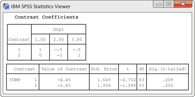
Some statistical software packages report the test statistics associated with contrasts as F statistics rather than t statistics. These F statistics are the squares of the t statistics described earlier. The associated P-values are for the two-sided alternatives.

Questions about population means are expressed as hypotheses about contrasts. A contrast should express a specific question that we have in mind when designing the study. When contrasts are formulated before seeing the data, inference about contrasts is valid whether or not the ANOVA H0 of equality of means is rejected. Because the F test answers a very general question, it is less powerful than tests for contrasts designed to answer specific questions. Specifying the important questions before the analysis is undertaken enables us to use this powerful statistical technique.
Apply Your Knowledge
Question 14.16
14.16 Define a contrast.
An ANOVA was run with five groups. Give the coefficients for the contrast that compares the average of the means of the first two groups with the average of the means of the last three groups.
Question 14.17
14.17 Find the standard error.
Refer to the previous exercise. Suppose that there are 11 observations in each group and that sp=6. Find the standard error for the contrast.
14.17
SEc=1.651446.
Question 14.18
14.18 Is the contrast significant?
Refer to the previous exercise. Suppose that the average of the first two groups minus the average of the last three groups is 3.5. State an appropriate null hypothesis for this comparison, find the test statistic with its degrees of freedom, and report the result.
Question 14.19
14.19 Give the confidence interval.
Refer to the previous exercise. Give a 95% confidence interval for the difference between the average of the means of the first two groups and the average of the means of the last three groups.
14.19
(0.1822, 6.8176).
Multiple comparisons
In many studies, specific questions cannot be formulated in advance of the analysis. If H0 is not rejected, we conclude that the population means are indistinguishable on the basis of the data given. On the other hand, if H0 is rejected, we would like to know which pairs of means differ. Multiple-comparisons methods address this issue. It is important to keep in mind that multiple-comparisons methods are commonly used only after rejecting the ANOVA H0.
multiple comparisons

Return once more to the reading comprehension study described in Case 14.2. We found in Example 14.15 (pages 734–735) that the means were not all the same (F=4.48, df=2 and 63, P=0.015).
EXAMPLE 14.22 A t Statistic to Compare Two Means
CASE 14.2 Refer to Figures 14.11 and 14.14 (pages 734 and 735). There are three pairs of population means. We can compare Groups 1 and 2, Groups 1 and 3, and Groups 2 and 3. For each of these pairs, we can write a t statistic for the difference in means. To compare Basal with DRTA (1 with 2), we compute
t12=ˉx1−ˉx2sp√1n1+1n2=41.05−46.736.31√122+122=−2.99
The subscripts on t specify which groups are compared.
Apply Your Knowledge
Question 14.20
CASE 14.214.20 Compare Basal with Strat.
Verify that t13=−1.69.
Question 14.21
CASE 14.214.21 Compare DRTA with Strat.
Verify that t23=1.29. (This is the same t that we used for the contrast ψ2=μ2−μ3 in Example 14.20.)
14.21
Using the same denominator of 1.90, t=(46.73−44.27)/1.90=1.29
These t statistics are very similar to the pooled two-sample t statistic for comparing two population means. The difference is that we now have more than two populations, so each statistic uses the pooled estimator sp from all groups rather than the pooled estimator from just the two groups being compared. This additional information about the common σ increases the power of the tests. The degrees of freedom for all of these statistics are DFE=63, those associated with sp.
Because we do not have any specific ordering of the means in mind as an alternative to equality, we must use a two-sided approach to the problem of deciding which pairs of means are significantly different.
Multiple Comparisons
To perform a multiple-comparisons procedure, compute t statistics for all pairs of means using the formula
tij=ˉxi−ˉxjsp√1ni+1nj
If
|tij|≥t**
we declare that the population means μi and μj are different. Otherwise, we conclude that the data do not distinguish between them. The value of t** depends on which multiple-comparisons procedure we choose.

One obvious choice for t** is the upper α/2 critical value for the t(DFE) distribution. This choice simply carries out as many separate significance tests of fixed level α as there are pairs of means to be compared. The procedure based on this choice is called the least-significant differences method, or simply LSD. LSD has some undesirable properties, particularly if the number of means being compared is large. Suppose, for example, that there are I=20 groups and we use LSD with α=0.05 . There are 190 different pairs of means. If we perform 190 t tests, each with an error rate of 5%, our overall error rate will be unacceptably large. We would expect about 5% of the 190 to be significant even if the corresponding population means are all the same. Because 5% of 190 is 9.5, we would expect 9 or 10 false rejections.
LSD method
The LSD procedure fixes the probability of a false rejection for each single pair of means being compared. It does not control the overall probability of some false rejection among all pairs. Other choices of t** control possible errors in other ways. The choice of t** is, therefore, a complex problem, and a detailed discussion of it is beyond the scope of this text. Many choices for t** are used in practice. One major statistical package allows selection from a list of more than a dozen choices.
We discuss only one of these, the Bonferroni method. Use of this procedure with α=0.05, for example, guarantees that the probability of any false rejection among all comparisons made is no greater than 0.05. This is much stronger protection than controlling the probability of a false rejection at 0.05 for each separate comparison.
Bonferroni method
EXAMPLE 14.23 Which Means Differ?
CASE 14.2 We apply the Bonferroni multiple-comparisons procedure with α=0.05 to the data from the new-product evaluation study in Example 14.15 (pages 734–735). The value of t** for this procedure (from software or special tables) is 2.46. The t statistic for comparing Basal with DRTA is t12=−2.99. Because |−2.99| is greater than 2.46, the value of t**, we conclude that the DRTA method produces higher reading comprehension scores than Basal.
Apply Your Knowledge
Question 14.22
CASE 14.214.22 Compare Basal with Strat.
The test statistic for comparing Basal with Strat is t13=−1.69. For the Bonferroni multiple-comparisons procedure with α=0.05, do you reject the null hypothesis that the population means for these two groups are different?
Question 14.23
CASE 14.214.23 Compare DRTA with Strat.
Answer the same question for the comparison of DRTA with Strat using the calculated value t23=1.29.
14.23
Because |1.29|<2.46, we fail to reject H0; we show no difference between DRTA and Strat with the Bonferroni multiple-comparisons procedure.
Usually, we use software to perform the multiple-comparisons procedure. The formats differ from package to package but they all give the same basic information.
EXAMPLE 14.24 Computer Output for Multiple Comparisons
eduprod
CASE 14.2 The output from SPSS for Bonferroni comparisons appears in Figure 14.17. The first line of numbers gives the results for comparing Basal with DRTA, Groups 1 and 2. The difference between the means is given as −5.682 with a standard error of 1.904. The P-value for the comparison is given under the heading “Sig.” The value is 0.012. Therefore, we could declare the means for Basal and DRTA to be different according to the Bonferroni procedure as long as we are using a value of α that is less than or equal to 0.012. In particular, these groups are significantly different at the overall α=0.05 level. The last two entries in the row give the Bonferroni 95% confidence interval. We discuss this later.
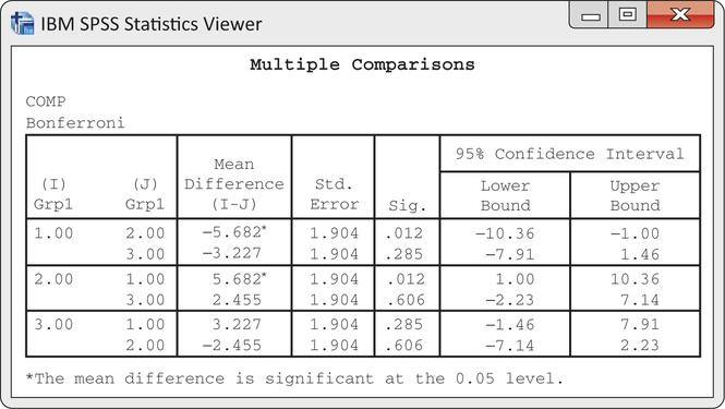
SPSS does not give the values of the t statistics for multiple comparisons. To compute them, simply divide the difference in the means by the standard error. For comparing Basal with DRTA, we have (as before)
t12=−5.6821.90=−2.99
Apply Your Knowledge
Question 14.24
CASE 14.214.24 Compare Basal with Strat.
Use the difference in means and the standard error reported in the output of Figure 14.17 to verify that t13=−1.69.
Question 14.25
CASE 14.214.25 Compare DRTA with Strat.
Use the difference in means and the standard error reported in the output of Figure 14.17 to verify that t23=1.29.
14.25
t23=2.455/1.90=1.29.
When there are many groups, the many results of multiple comparisons are difficult to describe. Here is one common format.
EXAMPLE 14.25 Displaying Multiple-Comparisons Results
CASE 14.2 Here is a table of the means and standard deviations for the three treatment groups. To report the results of multiple comparisons, use letters to label the means of pairs of groups that do not differ at the overall 0.05 significance level.
| Group | ˉx | s | n |
| Basal | 41.05A | 2.97 | 22 |
| DRTA | 46.73B | 2.65 | 22 |
| Strat | 44.27A,B | 3.34 | 22 |
Label A shows that Basal and Strat do not differ. Label B shows that DRTA and Strat do not differ. Because Basal and DRTA do not have a common label, they do differ.
The display in Example 14.25 shows that, at the overall 0.05 significance level, Basal does not differ from Strat and Strat does not differ from DRTA, yet Basal does differ from DRTA. These conclusions appear to be illogical. If μ1 is the same as μ3, and μ3 is the same as μ2, doesn’t it follow that μ1 is the same as μ2? Logically, the answer must be Yes.
This apparent contradiction points out the nature of the conclusions of tests of significance. A careful statement would say that we found significant evidence that Basal differs from DRTA and failed to find evidence that Basal differs from Strat or that Strat differs from DRTA. Failing to find strong enough evidence that two means differ doesn’t say that they are equal. It is very unlikely that any two methods of teaching reading comprehension would give exactly the same population means, but the data can fail to provide good evidence of a difference. This is particularly true in multiple-comparisons methods such as Bonferroni that use a single α for an entire set of comparisons.
Apply Your Knowledge
Question 14.26
14.26 Which means differ significantly?
Here is a table of means for a one-way ANOVA with four groups:
| Group | ˉx | s | n |
| Group 1 | 128.4 | 9.8 | 20 |
| Group 2 | 147.8 | 13.5 | 20 |
| Group 3 | 151.3 | 15.3 | 20 |
| Group 4 | 131.5 | 11.5 | 20 |
According to the Bonferroni multiple-comparisons procedure with α=0.05, the means for the following pairs of groups do not differ significantly: 1 and 4, 2 and 3. Mark the means of each pair of groups that do not differ significantly with the same letter. Summarize the results.
Question 14.27
14.27 The groups can overlap.
Refer to the previous exercise. Here is another table of means:
| Group | ˉx | s | n |
| Group 1 | 128.4 | 9.8 | 20 |
| Group 2 | 138.7 | 13.5 | 20 |
| Group 3 | 143.3 | 15.3 | 20 |
| Group 4 | 131.5 | 11.5 | 20 |
According to the Bonferroni multiple-comparisons procedure with α=0.05, the means for the following pairs of groups do not differ significantly: 1 and 2, 1 and 4, 2 and 3, 2 and 4. Mark the means of each pair of groups that do not differ significantly with the same letter. Summarize the results.
14.27
Groups 1 and 4 are marked A. Group 2 gets both A and B. Group 3 is marked B. Group 3 is the highest and is significantly higher than Groups 1 and 4. Group 2 is caught in between—it is not different from Group 3 nor is it different from Groups 1 and 4.
Simultaneous confidence intervals
One way to deal with these difficulties of interpretation is to give confidence intervals for the differences. The intervals remind us that the differences are not known exactly. We want to give simultaneous confidence intervals—that is, intervals for all the differences among the population means with, say, 95% confidence that all the intervals at once cover the true population differences. Again, there are many competing procedures—in this case, many methods of obtaining simultaneous intervals.
simultaneous confidence
intervals
Simultaneous Confidence Intervals for Differences between Means
Simultaneous confidence intervals for all differences μi−μj between population means have the form
(ˉxi−ˉxj)±t**sp√1ni+1nj
The critical values t** are the same as those used for the multiple comparisons procedure chosen.
The confidence intervals generated by a particular choice of t** are closely related to the multiple comparisons results for that same method. If one of the confidence intervals includes the value 0, then that pair of means will not be declared significantly different, and vice versa.
EXAMPLE 14.26 Software Output for Confidence Intervals
CASE 14.2 For simultaneous 95% Bonferroni confidence intervals, SPSS gives the output in Figure 14.17 for the data in Case 14.2. We are 95% confident that all three intervals simultaneously contain the true values of the population mean differences. After rounding the output, the confidence interval for the difference between the mean of the Basal group and the mean of the DRTA group is (−10.36, −1.00). This interval does not include zero, so we conclude that the DRTA method results in higher mean comprehension scores than the Basal method. This is the same conclusion we obtained from the significance test, but the confidence interval provides us with additional information about the size of the difference.
Apply Your Knowledge
Question 14.28
CASE 14.214.28 Confidence interval for Basal versus Strat.
Refer to the output in Figure 14.17. Give the Bonferroni 95% confidence interval for the difference between the mean comprehension score for the Basal method and the mean comprehension score for the Strat method. Be sure to round the numbers from the output in an appropriate way. Does the interval include 0?
Question 14.29
CASE 14.214.29 Confidence interval for DRTA versus Strat.
Refer to the previous exercise. Give the interval for comparing DRTA with Strat. Does the interval include 0?
14.29
(−2.23, 7.14). The interval includes 0, showing no significant difference between DRTA and Strat.
