15.2 Inference for Two-Way ANOVA
 This page includes Video Technology Manuals
Because two-way ANOVA breaks the FIT part of the model into three parts, corresponding to the two main effects and the interaction, inference for two-way ANOVA includes an F statistic for each of these effects. As with one-way ANOVA, the calculations are organized in an ANOVA table.
The ANOVA table for two-way ANOVA
The results of a two-way ANOVA are summarized in an ANOVA table based on splitting the total variation SST and the total degrees of freedom DFT among the two main effects and the interaction. When the sample size is the same for all groups, both the sums of squares (which measure variation) and the degrees of freedom add:
SST=SSA + SSB + SSAB + SSEDFT=DFA + DFB + DFAB + DFE

When the nij are not all equal, there are several ways to decompose SST, and the sums of squares may not add. Whenever possible, design studies with equal sample sizes to avoid these complications. We consider inference only for the equal-sample-size case.
The sums of squares are always calculated in practice by statistical software. From each sum of squares and its degrees of freedom, we find the mean square in the usual way:
mean square=sum of squaresdegrees of freedom
The significance of each of the main effects and the interaction is assessed by an F statistic that compares the variation due to the effect of interest with the within-group variation. Each F statistic is the mean square for the source of interest divided by MSE. Here is the general form of the two-way ANOVA table:
| Source | Degrees of freedom |
Sum of squares |
Mean square | F |
| A | I−1 | SSA | SSA/DFA | MSA/MSE |
| B | J−1 | SSB | SSB/DFB | MSB/MSE |
| AB | (I−1)(J−1) | SSAB | SSAB/DFAB | MSAB/MSE |
| Error | N−IJ | SSE | SSE/DFE | |
| Total | N−1 | SST | SST/DFT |
There are three null hypotheses in two-way ANOVA, with an F test for each. We can test for significance of the main effect of A, the main effect of B, and the AB interaction. It is generally good practice to examine the test for interaction first because the presence of a strong interaction may influence the interpretation of the main effects. Be sure to plot the means as an aid to interpreting the results of the significance tests.
Significance Tests in Two-Way ANOVA
To test the main effect of A, use the F statistic
FA=MSAMSE
To test the main effect of B, use the F statistic
FB=MSBMSE
To test the interaction of A and B, use the F statistic
FAB=MSABMSE
If the effect being tested is zero, the calculated F statistic has an F distribution with numerator degrees of freedom corresponding to the effect and denominator degrees of freedom equal to DFE. Large values of the F statistic lead to rejection of the null hypothesis. The P-value is the probability that a random variable having the corresponding F distribution is greater than or equal to the calculated value.
Apply Your Knowledge
Question 15.8
15.8 What’s wrong?
For each of the following, explain what is wrong and why.
- You should reject the null hypothesis that there is no interaction in a two-way ANOVA when the test statistic is small.
- Sums of squares are equal to mean squares divided by degrees of freedom.
- The significance tests for the main effects in a two-way ANOVA have a chi-square distribution when the null hypothesis is true.
- The estimate s2p is obtained by pooling the marginal sample variances.
Question 15.9
15.9 Customers’ preferences for packaging.
Exercise 15.2 (page 15-6) describes the setting for a two-way ANOVA design that compares different types of buyers (impulse or not) and the color of sales tags. Give the degrees of freedom for each of the F statistics that are used to test the main effects and the interaction for this problem.
15.9
For the tag color main effect, DF=3,130. For the impulse main effect, DF=1,130. For the interaction effect, DF=3,130.
Question 15.10
15.10 Comparing employee training programs.
Exercise 15.3 (pages 15-6 to 15-7) describes the setting for a two-way ANOVA design that compares employee training programs. Give the degrees of freedom for each of the F statistics that are used to test the main effects and the interaction for this problem.
Carrying out a two-way ANOVA
The following case illustrates how to do a two-way ANOVA. As with the one-way ANOVA, we focus our attention on interpretation of the computer output.


freqd
Does the frequency with which a supermarket product is offered at a discount affect the price that customers expect to pay for the product? Does the percent reduction also affect this expectation? These questions were examined by researchers in a study conducted on students enrolled in an introductory management course at a large midwestern university. For 10 weeks, 160 subjects received information about the products. The treatment conditions corresponded to the number of promotions (one, three, five, and seven) during this 10-week period, and the percent that the product was discounted (10%, 20%, 30%, and 40%). Ten students were randomly assigned to each of the 4×4=16 treatments.9 For our case study, we examine the data for two levels of promotions (1 and 3) and two levels of discount (40% and 20%). Thus, we have a two-way ANOVA with each of the factors having two levels and 10 observations in each of the four treatment combinations. Here are the data:
| Number of promotions |
Percent discount |
Expected price ($) | |||||||||
| 1 | 40 | 4.10 | 4.50 | 4.47 | 4.42 | 4.56 | 4.69 | 4.42 | 4.17 | 4.31 | 4.59 |
| 1 | 20 | 4.94 | 4.59 | 4.58 | 4.48 | 4.55 | 4.53 | 4.59 | 4.66 | 4.73 | 5.24 |
| 3 | 40 | 4.07 | 4.13 | 4.25 | 4.23 | 4.57 | 4.33 | 4.17 | 4.47 | 4.60 | 4.02 |
| 3 | 20 | 4.88 | 4.80 | 4.46 | 4.73 | 3.96 | 4.42 | 4.30 | 4.68 | 4.45 | 4.56 |
As usual we start our statistical analysis with a careful examination of the data.
EXAMPLE 15.11 Plotting the Data
freqd1
CASE 15.1 With 10 observations per treatment, we can plot the individual observations. To do this, we created an additional variable, “Comb,” that has four distinct values corresponding to the particular combination of the number of promotions and the discount. The value “d20-p1” corresponds to 20% discount with one promotion, and the values “d20-p3,” “d40-p1,” and “d40-p3” have similar interpretations. The data are plotted in Figure 15.5. The lines in the figure connect the four group means.
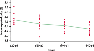
The spreads of the data within the groups are similar, and there are no outliers or other unusual patterns. That is, the conditions for ANOVA inference appear to be satisfied. The treatment means appear to differ.

freqd
Our second case study is a variation on the first. We use data from the experiment described in Case 15.1 but with different treatment combinations. Here are the data for the factor promotions at levels 1 and 5, and the factor discount at levels 30% and 10%:
| Number of promotions |
Percent discount |
Expected price ($) | |||||||||
| 1 | 30 | 3.57 | 3.77 | 3.90 | 4.49 | 4.00 | 4.66 | 4.48 | 4.64 | 4.31 | 4.43 |
| 1 | 10 | 5.19 | 4.88 | 4.78 | 4.89 | 4.69 | 4.96 | 5.00 | 4.93 | 5.10 | 4.78 |
| 5 | 30 | 3.90 | 3.77 | 3.86 | 4.10 | 4.10 | 3.81 | 3.97 | 3.67 | 4.05 | 3.67 |
| 5 | 10 | 4.31 | 4.36 | 4.75 | 4.62 | 3.74 | 4.34 | 4.52 | 4.37 | 4.40 | 4.52 |
Apply Your Knowledge
Question 15.11
CASE 15.215.11 Plot the data for Case 15.2.
Make a plot similar to the one given in Figure 15.5 for the levels of the factors given in Case 15.2. Connect the means with lines. Do the conditions for ANOVA inference appear to be met? Describe the pattern of the group means.
15.1
The d30-p1 group seems more spread out than the other 3 groups; also, the d10-p5 group has a low outlier. These concerns likely violate the conditions for ANOVA. The mean prices do seem different for the different promotion and discount combinations.
freq2
After looking at the data for Case 15.1 graphically, we proceed with numerical summaries.
EXAMPLE 15.12 Means and Standard Deviations
freqd1
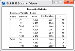
CASE 15.1 The software output in Figure 15.6 gives descriptive statistics for the data of Case 15.1. In the row with 1 under the heading “Promo” and 20 under the heading “Discount,” the mean of the 10 observations in this treatment combination is given as 4.689. The standard deviation is 0.2331. We would report these as 4.69 and 0.23. The next row gives results for one promotion and a 40% discount. The marginal results for all 20 students assigned to one promotion appear in the following “Total” row. The marginal standard deviation 0.2460 is not useful because it ignores the fact that the 10 observations for the 20% discount and the 10 observations for the 40% discount come from different populations. The overall mean for all 40 observations appears in the last row of the table. The standard deviations for the four groups are quite similar, and we have no reason to suspect a serious violation of the condition that the population standard deviations must all be the same.
Often, we display the means in a table similar to the following:
| Discount | |||
| Promotions | 20% | 40% | Total |
| 1 | 4.69 | 4.42 | 4.56 |
| 3 | 4.52 | 4.28 | 4.40 |
| Total | 4.61 | 4.35 | 4.48 |
In this table, the marginal means give us information about the main effects. When promotions are increased from one to three, the expected price drops from $4.56 to $4.40. Furthermore, when the discount is increased from 20% to 40%, the expected price drops from $4.61 to $4.35.
Numerical summaries with marginal means enable us to describe the main effects in a two-way ANOVA. For interactions, however, graphs are much better.
EXAMPLE 15.13 Plotting the group Means
freqd1
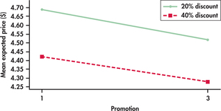
CASE 15.1 The means for the promotions and discount data of Case 15.1 are plotted in Figure 15.7. We have chosen to put the two values of promotion on the x axis. We see that the mean expected price for the 40% discount condition is consistently lower than the mean expected price for the 20% discount condition. Similarly, the means for three promotions are consistently less than the means for one promotion. The two lines are approximately parallel, suggesting that there is little interaction between promotion and discount in this example.
Apply Your Knowledge
Question 15.12
CASE 15.115.12 Group means in Excel output.
The first part of the Excel output in Figure 15.8 gives the group means and the marginal means for the data in Case 15.1. Find these means and display them in a table. Report them with the digits exactly as given in the output. Does Excel agree with the SPSS output in Figure 15.6?
Question 15.13
CASE 15.215.13 Numerical summaries for Case 15.2.
Find the means and standard deviations for each of the promotion-by-discount treatment combinations for the data in Case 15.2. Display the means in a table that also includes the marginal means. Plot the means and describe the main effects and the interaction. Do the standard deviations suggest that it is reasonable to pool the group standard deviations to get MSE?
15.13
We cannot pool the standard deviations because the largest s is more than twice the smallest s,0.38561>2(0.15202)=0.30404. There doesn’t appear to be an interaction. The expected price is higher for a 10% discount than for a 30% discount; the expected price is also higher with only 1 promotion compared with 5 promotions.
| Promotions | Discount | N | Mean | Standard Deviation |
| . | . | 40 | 4.357 | 0.45211 |
| . | 10 | 20 | 4.6565 | 0.34379 |
| . | 30 | 20 | 4.0575 | 0.33546 |
| 1 | . | 20 | 4.5725 | 0.45661 |
| 5 | . | 20 | 4.1415 | 0.33661 |
| 1 | 10 | 10 | 4.92 | 0.15202 |
| 1 | 30 | 10 | 4.225 | 0.38561 |
| 5 | 10 | 10 | 4.393 | 0.26854 |
| 5 | 30 | 10 | 3.89 | 0.16289 |
freqd2
Having examined the data carefully using numerical and graphical summaries, we are now ready to proceed with the statistical examination of the data using the two-way ANOVA model.
EXAMPLE 15.14 ANOVA Software Output
freqd1
CASE 15.1 Figure 15.8 gives the two-way ANOVA output from Minitab, Excel, SPSS, and SAS. Look first at the ANOVA table in the Minitab output. The form of the table is very similar to the general form of the two-way ANOVA table given on page 15-14. In place of A and B as the generic factors, the output gives the labels that we specified when we entered the data. We have main effects for “Discount” and “Promo.” The interaction between these two factors is labeled “Promo*Discount,” and the last two rows are “Error” and “Total.” The results of the significance tests are in the last two columns, labeled “F-Value” and “P-Value.” As expected, the interaction is not statistically significant (F=0.03,df=1 and 36,P=0.856). On the other hand, the main effects of discount (F=12.59,df=1 and 36,P=0.001) and promotion (F=4.54,df=1 and 36,P=0.040) are significant.
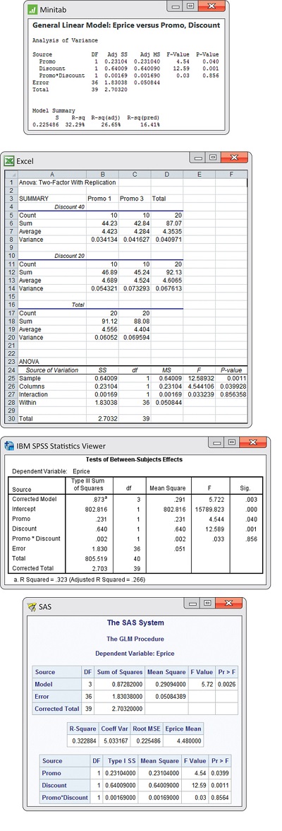
The statistical significance tests assure us that the differences that we saw in the graphical and numerical summaries can be distinguished from chance variation. We summarize as follows: When promotions are increased from one to three, the expected price drops from $4.56 to $4.40 (F=4.54, df=1 and 36,P=0.040). Furthermore, when the discount is increased from 20% to 40%, the expected price decreases from $4.61 to $4.35 (F=12.59, df=1 and 36,P=0.001).
Some software does not explicitly give s, the estimate of the parameter σ of our model. To find this, we take the square root of the mean square error, s=√0.0508=0.225.
Apply Your Knowledge
Question 15.14
CASE 15.115.14 Verify the ANOVA calculations.
Use the output in Figure 15.8 to verify that the four mean squares are obtained by dividing the corresponding sums of squares by the degrees of freedom. Similarly, show how each F statistic is obtained by dividing two of the mean squares.
Question 15.15
CASE 15.115.15 Compare software outputs.
Examine the outputs of Figure 15.8 from Minitab, Excel, SPSS, and SAS carefully. Write a short evaluation comparing the formats. Indicate which you prefer and why.
Question 15.16
CASE 15.215.16 Run the ANOVA for Case 15.2.
Analyze the data for Case 15.2 using the two-way ANOVA model and summarize the results.
freqd2