16.2 The Wilcoxon Signed Rank Test
 This page includes Video Technology Manuals
We use the one-sample t procedures for inference about the mean of one population or for inference about the mean difference in a matched pairs setting. We now meet a rank test for matched pairs and single samples. The matched pairs setting is more important because good studies are generally comparative.
EXAMPLE 16.6 Loss of Product Value
vitc
Food products are often enriched with vitamins and other supplements. Does the level of a supplement decline over time so that the user receives less than the manufacturer intended? Here are data on the vitamin C levels (milligrams per 100 grams) in wheat soy blend, a flour-like product supplied by international aid programs mainly for feeding children. The same nine bags of blend were measured at the factory and five months later in Haiti.10
| Bag | 1 | 2 | 3 | 4 | 5 | 6 | 7 | 8 | 9 |
| Factory | 45 | 32 | 47 | 40 | 38 | 41 | 37 | 52 | 37 |
| Haiti | 38 | 40 | 35 | 38 | 34 | 35 | 38 | 38 | 40 |
| Difference | 7 | −8 | 12 | 2 | 4 | 6 | −1 | 14 | −3 |
We suspect that vitamin C levels are generally higher at the factory than they are five months later. We would like to test the hypotheses
- H0: vitamin C has the same distribution at both times
- Ha: vitamin C is systematically higher at the factory
Because these are matched pairs data, we base our inference on the differences.
Positive differences in Example 16.6 indicate that the vitamin C level of a bag was higher at the factory than in Haiti. If factory values are generally higher, the positive differences should be farther from zero in the positive direction than the negative differences are in the negative direction. Therefore, we compare the absolute values of the differences—that is, their magnitudes without a sign. Here they are, with boldface indicating the positive values:
absolute value
| 7 | 8 | 12 | 2 | 4 | 6 | 1 | 14 | 3 |
Arrange the absolute values in increasing order and assign ranks, keeping track of which values were originally positive. Tied values receive the average of their ranks. If there are zero differences, discard them before ranking. In our example, there are no zeros and no ties.
| Absolute value | 1 | 2 | 3 | 4 | 6 | 7 | 8 | 12 | 14 |
| Rank | 1 | 2 | 3 | 4 | 5 | 6 | 7 | 8 | 9 |
The test statistic is the sum of the ranks of the positive differences. This is the Wilcoxon signed rank statistic. Its value here is W+=34. (We could equally well use the sum of the ranks of the negative differences, which is 11.)
The Wilcoxon Signed Rank Test for Matched Pairs
Draw an SRS from a population for a matched pairs study and take the differences in responses within pairs. Remove all zero differences, so that n nonzero differences remain. Rank the absolute values of these differences. The sum W+ of the ranks for the positive differences is the Wilcoxon signed rank statistic.
If the distribution of the responses is not affected by the different treatments within pairs, then W+ has mean
μW+=n(n+1)4
and standard deviation
σW+=√n(n+1)(2n+1)24
The Wilcoxon signed rank test rejects the hypothesis that there are no systematic differences within pairs when the rank sum W+ is far from its mean.
Apply Your Knowledge
Question 16.27
16.27 Service and food provided by top 25 spas.
The readers’ poll in Condé Nast Traveler magazine that ranked 100 top resort spas and that was described in Exercise 16.1 also reported scores on service and on food. Here are the scores for a random sample of seven spas that ranked in the top 25.
| Spa | 1 | 2 | 3 | 4 | 5 | 6 | 7 |
| Service | 89.6 | 89.8 | 87.3 | 94.2 | 95.8 | 87.9 | 91.0 |
| Food | 83.1 | 88.1 | 85.8 | 92.9 | 95.7 | 80.7 | 83.6 |
Is service more important than food for a top ranking? Formulate this question in terms of null and alternative hypotheses. Then compute the differences and find the value of the Wilcoxon signed rank statistic, W+.
16.27
H0: There is no difference in the distribution between service and food scores. Ha: Service scores are systematically higher than food scores. W+=28.
spas3
Question 16.28
16.28 Scores for the next 25 spas.
Refer to the previous exercise. Here are the scores for a random sample of seven spas that ranked between 26 and 50.
| Spa | 1 | 2 | 3 | 4 | 5 | 6 | 7 |
| Service | 90.6 | 87.2 | 95.0 | 88.4 | 91.5 | 88.2 | 91.2 |
| Food | 86.6 | 74.4 | 89.1 | 81.0 | 85.7 | 83.2 | 93.1 |
Answer the questions from the previous exercise for this setting.
spas4
EXAMPLE 16.7 Loss of Product Value: Rank Test
vitc
In the vitamin loss study of Example 16.6, n=9. If the null hypothesis (no systematic loss of vitamin C) is true, the mean of the signed rank statistic is
μW+=n(n+1)4=(9)(10)4=22.5
Our observed value W+=34 is somewhat larger than this mean. The one-sided P-value is P(W+≥34).
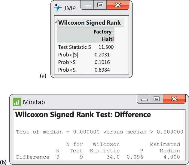
Figure 16.6 displays the output of two statistical programs. We see from Figure 16.6(a) that the one-sided P-value is P=0.1016. JMP reports a statistic S as being 11.5. This is simply the difference between W+ and μW+. This small sample does not give convincing evidence of vitamin loss.
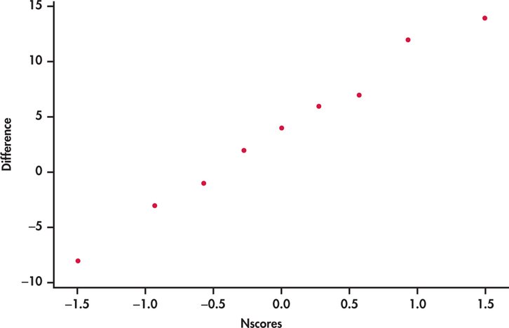
In fact, the Normal quantile plot in Figure 16.7 shows that the differences are reasonably Normal. We could use the paired-sample t to get a similar conclusion (t=1.5595, df=8, P=0.0787). The t test has a slightly lower P-value because it is somewhat more powerful than the rank test when the data are actually Normal.
Although we emphasize the matched pairs setting, W+ can also be applied to a single sample. It then tests the hypothesis that the population median is zero. For matched pairs, we are testing that the median of the differences is zero. To test the hypothesis that the population median has a specific value m, apply the test to the differences Xi=m.
The Normal approximation
The distribution of the signed rank statistic when the null hypothesis (no difference) is true becomes approximately Normal as the sample size becomes large. We can then use Normal probability calculations (with the continuity correction) to obtain approximate P-values for W+. Let’s see how this works in the loss of product value example, even though n=9 is certainly not a large sample.
EXAMPLE 16.8 Loss of Product Value: Normal Approximation
vitc
For n=9 observations, we saw in Example 16.7 that μW+=22.5. The standard deviation of W+ under the null hypothesis is
σW+=√n(n+1)(2n+1)24=√(9)(10)(19)24=√71.25=8.441
The continuity correction calculates the P-value P(W+≥34) as P(W+≥33.5), treating the value W+=34 as occupying the interval from 33.5 to 34.5. We find the Normal approximation for the P-value by standardizing and using the standard Normal table:
P(W+≥33.5)=P(W+−22.58.441≥33.5−22.58.441)=P(Z≥1.303)=0.0968
Despite the small sample size, the Normal approximation gives a result quite close to the exact value P=0.1016. The Minitab output in Figure 16.6(b) gives P=0.096 based on a Normal calculation rather than the table.
Apply Your Knowledge
Question 16.29
16.29 Significance test for top-ranked spas.
Refer to Exercise 16.27 (page 16-17). Find μW+, σW+, and the Normal approximation for the P-value for the Wilcoxon signed rank test.
16.29
μW+=14, σW+=5.9161. z=2.28, P-value=0.0113.
spas3
Question 16.30
16.30 Significance test for lower-ranked spas.
Refer to Exercise 16.28 (page 16-17). Find μW+, σW+, and the Normal approximation for the P-value for the Wilcoxon signed rank test.
spas4
Ties
Ties among the absolute differences are handled by assigning average ranks. A tie within a pair creates a difference of zero. Because these are neither positive nor negative, we drop such pairs from our sample. As in the case of the Wilcoxon rank sum, ties complicate finding a P-value. There is no longer a usable exact distribution for the signed rank statistic W+, and the standard deviation σW+ must be adjusted for the ties before we can use the Normal approximation. Software will do this. Here is an example.
EXAMPLE 16.9 Two Rounds of Golf Scores
golf
Here are the golf scores of 12 members of a college women’s golf team in two rounds of tournament play. (A golf score is the number of strokes required to complete the course, so that low scores are better.)
| Player | 1 | 2 | 3 | 4 | 5 | 6 | 7 | 8 | 9 | 10 | 11 | 12 |
| Round 2 | 94 | 85 | 89 | 89 | 81 | 76 | 107 | 89 | 87 | 91 | 88 | 80 |
| Round 1 | 89 | 90 | 87 | 95 | 86 | 81 | 102 | 105 | 83 | 88 | 91 | 79 |
| Difference | 5 | −5 | 2 | −6 | −5 | −5 | 5 | −16 | 4 | 3 | −3 | 1 |
Negative differences indicate better (lower) scores on the second round. We see that six of the 12 golfers improved their scores. We would like to test the hypotheses that in a large population of collegiate woman golfers
- H0: scores have the same distribution in rounds 1 and 2
- Ha: scores are systematically lower or higher in round 2
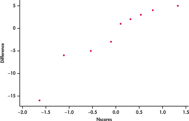
A Normal quantile plot of the differences (Figure 16.8) shows some irregularity and a low outlier. We will use the Wilcoxon signed rank test.
The absolute values of the differences, with boldface indicating those that were negative, are
| 5 | 5 | 2 | 6 | 5 | 5 | 5 | 16 | 4 | 3 | 3 | 1 |
Arrange these in increasing order and assign ranks, keeping track of which values were originally negative. Tied values receive the average of their ranks.
| Absolute value | 1 | 2 | 3 | 3 | 4 | 5 | 5 | 5 | 5 | 5 | 6 | 16 |
| Rank | 1 | 2 | 3.5 | 3.5 | 5 | 8 | 8 | 8 | 8 | 8 | 11 | 12 |
The Wilcoxon signed rank statistic is the sum of the ranks of the negative differences. (We could equally well use the sum of the ranks of the positive differences.) Its value is W+=50.5.
EXAMPLE 16.10 Software Results for Golf Scores
golf
Here are the two-sided P-values for the Wilcoxon signed rank test for the golf score data from several statistical programs:
| Program | P-value |
| Minitab | P=0.388 |
| JMP | P=0.388 |
| SPSS | P=0.363 |
All lead to the same practical conclusion: these data give no evidence for a systematic change in scores between rounds. However, the P-values reported differ a bit from program to program. The reason for the variations is that the programs use slightly different versions of the approximate calculations needed when ties are present. The exact result depends on which of these variations the programmer chooses to use.
For these data, the matched pairs t test gives t=0.9314 with P=0.3716. Once again, t and W+ lead to the same conclusion.