16.3 The Kruskal-Wallis Test
 This page includes Video Technology Manuals
We have now considered alternatives to the paired-sample and two-sample t tests for comparing the magnitude of responses to two treatments. To compare more than two treatments, we use one-way analysis of variance (ANOVA) if the distributions of the responses to each treatment are at least roughly Normal and have similar spreads. What can we do when these distribution requirements are violated?
EXAMPLE 16.11 Weeds and Corn Yield
weeds
Lamb’s-quarter is a common weed that interferes with the growth of corn. A researcher planted corn at the same rate in 16 small plots of ground and then randomly assigned the plots to four groups. He weeded the plots by hand to allow a fixed number of lamb’s-quarter plants to grow in each meter of corn row. These numbers were zero, one, three, and nine in the four groups of plots. No other weeds were allowed to grow, and all plots received identical treatment except for the weeds. Here are the yields of corn (bushels per acre) in each of the plots:14
| Weeds per meter |
Corn yield |
Weeds per meter |
Corn yield |
Weeds per meter |
Corn yield |
Weeds per meter |
Corn yield |
| 0 | 166.7 | 1 | 166.2 | 3 | 158.6 | 9 | 162.8 |
| 0 | 172.2 | 1 | 157.3 | 3 | 176.4 | 9 | 142.4 |
| 0 | 165.0 | 1 | 166.7 | 3 | 153.1 | 9 | 162.7 |
| 0 | 176.9 | 1 | 161.1 | 3 | 156.0 | 9 | 162.4 |
The summary statistics are
| Weeds | n | Mean | Standard deviation |
| 0 | 4 | 170.200 | 5.422 |
| 1 | 4 | 162.825 | 4.469 |
| 3 | 4 | 161.025 | 10.493 |
| 9 | 4 | 157.575 | 10.118 |

The sample standard deviations do not satisfy our rule of thumb that for safe use of ANOVA the largest should not exceed twice the smallest. A careful look at the data suggests that there may be some outliers. These are the correct yields for their plots, so we have no justification for removing them. Let’s use a rank test that is not sensitive to outliers.
Hypotheses and assumptions
The ANOVA F test concerns the means of the several populations represented by our samples. For Example 16.11, the ANOVA hypotheses are
- H0:μ0=μ1=μ3=μ9
- Ha: not all four means are equal
Here, μ0 is the mean yield in the population of all corn planted under the conditions of the experiment with no weeds present. The data should consist of four independent random samples from the four populations, all Normally distributed with the same standard deviation.
Kruskal-Wallis test
The Kruskal-Wallis test is a rank test that can replace the ANOVA F test. The assumption about data production (independent random samples from each population) remains important, but we can relax the Normality assumption. We assume only that the response has a continuous distribution in each population. The hypotheses tested in our example are
- H0: yields have the same distribution in all groups
- Ha: yields are systematically higher in some groups than in others
If all the population distributions have the same shape (Normal or not), these hypotheses take a simpler form. The null hypothesis is that all four populations have the same median yield. The alternative hypothesis is that not all four median yields are equal.
The Kruskal-Wallis test
Recall the analysis of variance idea: we write the total observed variation in the responses as the sum of two parts, one measuring variation among the groups (sum of squares for groups, SSG) and one measuring variation among individual observations within the same group (sum of squares for error, SSE). The ANOVA F test rejects the null hypothesis that the mean responses are equal in all groups if SSG is large relative to SSE.
The idea of the Kruskal-Wallis rank test is to rank all the responses from all groups together and then apply one-way ANOVA to the ranks rather than to the original observations. If there are N observations in all, the ranks are always the whole numbers from 1 to N. The total sum of squares for the ranks is, therefore, a fixed number no matter what the data are. So we do not need to look at both SSG and SSE. Although it isn’t obvious without some unpleasant algebra, the Kruskal-Wallis test statistic is essentially just SSG for the ranks. We give the formula, but you should rely on software to do the arithmetic. When SSG is large, that is evidence that the groups differ.
The Kruskal-Wallis Test
Draw independent SRSs of sizes n1, n2, …, nI from I populations. There are N observations in all. Rank all N observations and let Ri be the sum of the ranks for the ith sample. The Kruskal-Wallis statistic is
H=[12N(N+1)∑R2ini]−3(N+1)
When the sample sizes ni are large and all I populations have the same continuous distribution, H has approximately the chi-square distribution with I−1 degrees of freedom.
The Kruskal-Wallis test rejects the null hypothesis that all populations have the same distribution when H is large.
We now see that, like the Wilcoxon rank sum statistic, the Kruskal-Wallis statistic is based on the sums of the ranks for the groups we are comparing. The more different these sums are, the stronger is the evidence that responses are systematically larger in some groups than in others.
The exact distribution of the Kruskal-Wallis statistic H under the null hypothesis depends on all the sample sizes n1 to nI, so tables are awkward. The calculation of the exact distribution is so time-consuming for all but the smallest problems that even most statistical software uses the chi-square approximation to obtain P-values. As usual, there is no usable exact distribution when there are ties among the responses. We again assign average ranks to tied observations.
EXAMPLE 16.12 Perform the Significance Test
weeds
In Example 16.11, there are I=4 populations and N=16 observations. The sample sizes are equal, ni=4. The 16 observations arranged in increasing order, with their ranks, are
| Yield | 142.4 | 153.1 | 156.0 | 157.3 | 158.6 | 161.1 | 162.4 | 162.7 |
| Rank | 1 | 2 | 3 | 4 | 5 | 6 | 7 | 8 |
| Yield | 162.8 | 165.0 | 166.2 | 166.7 | 166.7 | 172.2 | 176.4 | 176.9 |
| Rank | 9 | 10 | 11 | 12.5 | 12.5 | 14 | 15 | 16 |
There is one pair of tied observations. The ranks for each of the four treatments are
| Weeds | Ranks | Rank sums | |||
| 0 | 10 | 12.5 | 14 | 16 | 52.5 |
| 1 | 4 | 6 | 11 | 12.5 | 33.5 |
| 3 | 2 | 3 | 5 | 15 | 25.0 |
| 9 | 1 | 7 | 8 | 9 | 25.0 |
The Kruskal-Wallis statistic is, therefore,
H=[12N(N+1)∑R2ini]−3(N+1)=12(16)(17)(52⋅524+33⋅524+2524+2524)−(3)(17)=12272(1282.125)−515.56
Referring to the table of chi-square critical points (Table F) with df=3, we find that the P-value lies in the interval 0.10<P<0.15. This small experiment suggests that more weeds decrease yield but does not provide convincing evidence that weeds have an effect.
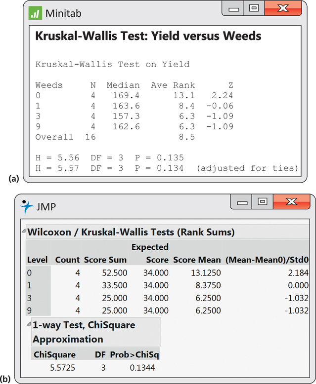
Figure 16.9 displays the output from Minitab and JMP for the analysis of the data in Example 16.12. Minitab gives the H statistic adjusted for ties as H=5.57 with 3 degrees of freedom and P=0.134. JMP reports a chi-square statistic with 3 degrees of freedom and P=0.1344. All agree that there is not sufficient evidence in the data to reject the null hypothesis that the number of weeds per meter has no effect on the yield.