17.1 The Logistic Regression Model
In general, the data for simple logistic regression are n independent cases, each consisting of a value of the explanatory variable x and either a success or a failure for that trial. For example, x may be the salary amount, and “success” means that this applicant accepted the job offer. Every observation may have a different value of x.
To introduce logistic regression, however, it is convenient to start with the special case in which the explanatory variable x is also a yes-or-no variable. The data then contain a number of outcomes (success or failure) for each of the two values of x. There are also just two values of p, one for each value of x. Assuming the count of successes for each value of x has a binomial distribution, we are on familiar ground as described in Chapters 5 and 8. Here is an example.


What are the factors that affect a customer's tipping behavior? Studies have shown that a server's gender and various aspects of a server's appearance have an effect on tipping, unrelated to the quality of service. Some of these same studies have shown that the effect is different for male and female customers.
Because the color red has been shown to increase the physical attractiveness of women, a group of researchers decided to see if the color of clothing a female server wears has an effect on the tipping behavior.2 Although they considered both male and female customers, we focus on the 418 male customers in the study.
The response variable is whether or not the male customer left a tip. The explanatory variable is whether the female server wore a red top or not. Let's express this condition numerically using an indicator variable,
x={1if the server wore a red top0if the server wore a different colored top
The female servers in the study wore a red top for 69 of the customers and wore a different colored top for the other 349.
The probability that a randomly chosen customer will tip has two values, p1 for those whose server wore a red top and p0 for those whose server wore a different colored top. The number of customers who tipped a server wearing red top has the binomial distribution B(69,p1). The number of customers who tipped a server wearing a different color top has the B(349,p0) distribution.
Binomial distributions and odds
We begin with a review of some ideas associated with binomial distributions.
EXAMPLE 17.1 Proportion of Tippers
red
CASE 17.1 In Chapter 8, we used sample proportions to estimate population proportions. For this study, 40 of the 69 male customers tipped a server who was wearing red and 130 of the 349 customers tipped a server who was wearing a different color. Our estimates of the two population proportions are
red:ˆp1=4069=0.5797
and
not red:ˆp0=130349=0.3725
That is, we estimate that 58.0% of the male customers will tip if the server wears red, and 37.3% of the male customers will tip if the server wears a different color.

Logistic regression works with odds rather than proportions. The odds are the ratio of the proportions for the two possible outcomes. If p is the probability of a success, then 1−p is the probability of a failure, and
odds=p1−p=probability of successprobability of failure
A similar formula for the sample odds is obtained by substituting ˆp for p in this expression.
EXAMPLE 17.2 Odds of Tipping
CASE 17.1 The proportion of tippers among male customers who have a server wearing red is ˆp1=0.5797, so the proportion of male customers who are not tippers when their server wears red is
1−ˆp1=1−0.5797=0.4203
The estimated odds of a male customer tipping when the server wears red are, therefore,
odds=ˆp11−ˆp1=0.57971−0.5797=1.3793
For the case when the server does not wear red, the odds are
odds=ˆp01−ˆp0=0.37251−0.3725=0.5936
When people speak about odds, they often round to integers or fractions. Because 1.3793 is approximately 7/5, we could say that the odds that a male customer tips when the server wears red are 7 to 5. In a similar way, we could describe the odds that a male customer does not tip when the server wears red as 5 to 7.
Apply Your Knowledge
Question 17.1
17.1 Energy drink commercials.
A study was designed to compare Red Bull energy drink commercials. Each participant was shown the commercials, A and B, in random order and asked to select the better one. There were 140 women and 130 men who participated in the study. Commercial A was selected by 65 women and by 67 men. Find the odds of selecting Commercial A for the men. Do the same for the women.
17.1
For men: the percent who chose Commercial A is 0.5154; the percent who chose Commercial B is 0.4846. The odds are 1.0636. For women: the percent who chose Commercial A is 0.4643; the percent who chose Commercial B is 0.5357. The odds are 0.8667.
Question 17.2
17.2 Use of audio/visual sharing through social media.
In Case 8.3 (page 438), we studied data on large and small food and beverage companies and the use of audio/visual sharing through social media. Here are the data:
| Observed numbers of companies | |||
| Use A/V sharing | |||
| Size | Yes | No | Total |
| Small | 150 | 28 | 178 |
| Large | 27 | 25 | 52 |
| Total | 177 | 53 | 230 |
What proportion of the small companies use audio/visual sharing? What proportion of the large companies use audio/visual sharing? Convert each of these proportions to odds.
Model for logistic regression
In Chapter 8, we learned how to compare the proportions of two groups (such as large and small companies) using z tests and confidence intervals. Simple logistic regression is another way to make this comparison, but it extends to more general settings with a success-or-failure response variable.
In simple linear regression we modeled the mean μ of the response variable y as a linear function of the explanatory variable: μ+β0+β1x. When y is just 1 or 0 (success or failure), the mean is the probability p of a success. Simple logistic regression models the mean p in terms of an explanatory variable x. We might try to relate p and x as in simple linear regression: p=β0+β1x. Unfortunately, this is not a good model. Whenever β1≠0, extreme values of x will give values of β0+β1x that fall outside the range of possible values of p, 0≤p≤1.
log odds or logit
The logistic regression model removes this difficulty by working with the natural logarithm of the odds. We use the term log odds or logit for this transformation of p. We model the log odds as a linear function of the explanatory variable:
log(p1−p)=β0+β1x
As p moves from 0 to 1, the log odds move through all negative and positive numerical values. Here is a summary of the logistic regression model.
Simple Logistic Regression Model
The statistical model for simple logistic regression is
log(p1−p)=β0+β1x
where p is a binomial proportion and x is the explanatory variable. The parameters of the logistic model are β0 and β1.
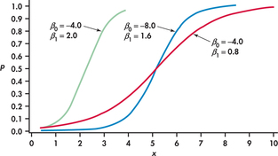
Figure 17.1 graphs the relationship between p and x for some different values of β0 and β1. The logistic regression model uses natural logarithms. There are tables of natural logarithms and most calculators have a built-in function for the natural logarithm, often labeled “ln.”
Returning to the tipping study, for servers wearing red we have
log(odds)=log(1.3793)=0.3216
and for servers not wearing red we have
log(odds)=log(0.5936)=−0.5215
Verify these results with your calculator, remembering that “log” in these equations is the natural logarithm.
Apply Your Knowledge
Question 17.3
17.3 Log odds choosing Commercial A.
Refer to Exercise 17.1. Find the log odds for the men and the log odds for the women choosing Commercial A.
17.3
For men: 0.06166. For women:−0.14306.
Question 17.4
17.4 Log odds for use of audio/visual sharing.
Refer to Exercise 17.2. Find the log odds for the small and large companies.
Fitting and interpreting the logistic regression model
We must now fit the logistic regression model to data. In general, the data consist of n observations on the explanatory variable x, each with a success-or-failure response. Our tipping example has an indicator (0 or 1) explanatory variable. Logistic regression with an indicator explanatory variable is a special case but is important in practice. We use this special case to understand a little more about the model.
EXAMPLE 17.3 Logistic model for Tipping Behavior
CASE 17.1 In the tipping example, there are n=418 observations. The explanatory variable is whether the server wore a red top or not, which we coded using an indicator variable with values x=1 for servers wearing red and x=0 for servers wearing a different color. There are 69 observations with x=1 and 349 observations with x=0. The response variable is also an indicator variable: y=1 if the customer left a tip and y=0 if not. The model says that the probability p of leaving a tip depends on the color of the server's top (x=1 or x=0). There are two possible values for p—say, p1 for servers wearing red and p0 for servers wearing a different color. The model says that for servers wearing red
log(p11−p1)=β0+β1
and for servers wearing a different color
log(p01−p0)=β0
Note that there is a β1 term in the equation for servers wearing red because x=1, but it is missing in the equation for servers wearing a different color because x=0.
In general, the calculations needed to find the estimates b0 and b1 for the parameters β0 and β1 are complex and require the use of software. When the explanatory variable has only two possible values, however, we can easily find the estimates. This simple framework also provides a setting where we can learn what the logistic regression parameters mean.
EXAMPLE 17.4 Parameter Estimates for Tipping Behavior
CASE 17.1 For the tipping example, we found the log odds for servers wearing red,
log(ˆp11−ˆp1)=0.3216
and for servers wearing a different color,
log(ˆp01−ˆp0)=−0.5215
To find estimates b0 and b1 of the model parameters β0 and β1 we match the two model equations in Example 17.3 with the corresponding data equations. Because
log(p01−p0)=β0andlog(ˆp01−ˆp0)=−0.5215
the estimate b0 of the intercept is simply the logs odds ) for servers wearing a different color,
b0=−0.5215
Similarly, the estimated slope is the difference between the log(odds) for servers wearing red and the log(odds) for servers wearing a different color,
b0=0.3216−(−0.5215)=0.8431
The fitted logistic regression model is
log(odds)=−0.5215+0.8431x
The slope in this logistic regression model is the difference between the log( odds ) for servers wearing red and the log(odds ) for servers wearing a different color. Most people are not comfortable thinking in the log(odds) scale, so interpretation of the results in terms of the regression slope is difficult.
EXAMPLE 17.5 Transforming Estimates to the Odds Scale
CASE 17.1 To get to the odds scale, we take the exponential of the log(odds). Based on the parameter estimates in Example 17.4,
odds=e−0.5215+0.8431x=e−0.5215×e0.8431x
From this, the ratio of the odds for a server wearing red (x=1) and for a server wearing a different color (x=0) is
oddsredoddsother=e0.8431=2.324
odds ratio
The transformation e0.8431 undoes the natural logarithm and transforms the logistic regression slope into an odds ratio, in this case, the comparison of odds that a male customer tips when a server is wearing red to the odds that a male customer tips when a server is wearing a different color. In other words, we can multiply the odds of tipping when a server wears a different color by the odds ratio to obtain the odds of tipping for a server wearing red:
oddsred=2.324×oddsother
In this case, the odds of tipping when a server wears red are about 2.3 times the odds when a server wears a different color.
Notice that we have chosen the coding for the indicator variable so that the regression slope is positive. This will give an odds ratio that is greater than 1. Had we coded servers wearing a different color as 1 and servers wearing red as 0, the sign of the slope would be reversed, and the fitted equation would be log(odds)=0.3216−0.8431x, and the odds ratio would be e−0.8431=0.430. The odds of tipping for servers wearing a different color are roughly 43% of the odds for servers wearing red.
Of course, it is often the case that the explanatory variable is quantitative rather than an indicator variable. We must then use software to fit the logistic regression model. Here is an example.
EXAMPLE 17.6 Will a Movie Be Profitable?
movprof
The MOVIES data set (described on page 550) includes both the movie's budget and the total U.S. revenue. For this example, we classify each movie as “profitable” (y=1) if U.S. revenue is larger than the budget and nonprofitable (y=0) otherwise. This is our response variable.
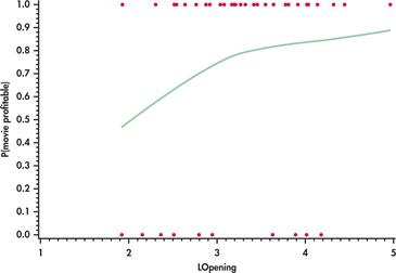
The data set contains several explanatory variables, but we focus here on the natural logarithm of the opening-weekend revenue, LOpening. Figure 17.2 is a scatterplot of the data with a scatterplot smoother (page 68). The probability that a movie is profitable increases with the log opening weekend revenue. Because an S-shaped curve like those in Figure 17.1 is suggested by the smoother, we fit the logistic regression model
log(p1−p)=β0+β1x
where p is the probability that the movie is profitable and x is the log opening-weekend revenue. The model for estimated log odds fitted by software is
log(odds)=b0+b1x=−1.41+0.781x
The estimated odds ratio is eb1=2.184. This means that if opening-weekend revenue x were roughly e1=2.72 times larger (for example, $18.1 million to $49.2 million), the odds that the movie will be profitable increase by 2.2 times.
Apply Your Knowledge
Question 17.5
17.5 Fitted model for energy drink commercials.
Refer to Exercise 17.1 and 17.3. Find the estimates b0 and b1 and give the fitted logistic model. What is the estimated odds ratio for a male to choose Commercial A(x=1) versus a female to choose Commercial A(x=0)?
17.5
b0=−0.14306, b1=0.20472.log(odds)=−0.14306+0.20472x.The odds ratio is 1.227.
Question 17.6
17.6 Fitted model for use of audio/video sharing.
Refer to Exercise 17.2 and 17.4. Find the estimates b0 and b1 and give the fitted logistic model. What is the estimated odds ratio for small (x=1) versus large (x=0) companies?
Question 17.7
17.7 Interpreting an odds ratio.
If we apply the exponential function to the fitted model in Example 17.6, we get
odds=e−1.41+0.781x=e−1.41×e0.781x
Show that for any value of the quantitative explanatory variable x, the odds ratio for increasing x by 1,
oddsx+1oddsx
is e0.781=2.184. This justifies the interpretation given at the end of Example 17.6.
17.7
oddsx+1oddsx=e−1⋅41+0⋅781(x+1)e−1⋅41+0⋅781x=e0⋅781xe0⋅781e0⋅781x=e0.781=2.184⋅
The odds ratio interpretation of the estimated slope parameter is a very attractive feature of the logistic regression model. The health sciences, for example, have used this model extensively to identify risk factors for disease and illness. There are other statistical models, such as probit regression, that describe binary responses, but none of them has this interpretation.
probit regression