17.2 Inference for Logistic Regression
Statistical inference for logistic regression with one explanatory variable is similar to statistical inference for simple linear regression. We calculate estimates of the model parameters and standard errors for these estimates. Confidence intervals are formed in the usual way, but we use standard Normal z*-values rather than critical values from the t distributions. The ratio of the estimate to the standard error is the basis for hypothesis tests.
Wald statistic
The statistic z is sometimes called the Wald statistic. Output from some statistical software reports the significance test result in terms of the square of the z statistic.
X2=z2
This statistic is called a chi-square statistic. When the null hypothesis is true, it has a distribution that is approximately a χ2 distribution with one degree of freedom, and the P-value is calculated as P(χ2≥X2). Because the square of a standard Normal random variable has a χ2 distribution with one degree of freedom, the z statistic and the chi-square statistic give the same results for statistical inference.

Confidence Intervals and Significance Tests for Logistic Regression
An approximate level C confidence interval for the slope β1 in the logistic regression model is
b1±z*SEb1
The ratio of the odds for a value of the explanatory variable equal to x+1 to the odds for a value of the explanatory variable equal to x is the odds ratio eβ1. A level C confidence interval for the odds ratio is obtained by transforming the confidence interval for the slope,
(eb1−z*SEb1,eb1+z*SEb1)
In these expressions z* is the standard Normal critical value with area C between −z* and z*.
To test the hypothesis H0:β1=0, compute the test statistic
X2=(b1SEb1)2
In terms of a random variable χ2 having the χ2 distribution with one degree of freedom, the P-value for a test of H0 against Ha:β1≠0 is approximately P(χ2≥X2).
We have expressed the null hypothesis in terms of the slope β1 because this form closely resembles what we studied in simple linear regression. In many applications, however, the results are expressed in terms of the odds ratio. A slope of 0 is the same as an odds ratio of 1, so we often express the null hypothesis of interest as “the odds ratio is 1.” This means that the two odds are equal and the explanatory variable is not useful for predicting the odds.
EXAMPLE 17.7 Computer Output for Tipping Study
red
CASE 17.1 Figure 17.3 gives the output from Minitab and SAS for the tipping study. The parameter estimates match those we calculated in Example 17.4. The standard errors are 0.1107 and 0.2678. A 95% confidence interval for the slope is
b1±z*SEb1=0.8431±(1.96)(0.2678)=0.8431±0.5249
We are 95% confident that the slope is between 0.3182 and 1.368. Both Minitab and SAS output provide the odds ratio estimate and 95% confidence interval. If this interval is not provided, it is easy to compute from the interval for the slope β1:
(eb1−z*SEb1,eb1+z*SEb1)=(e0.3182⋅e1.368)=(1.375,3.927)
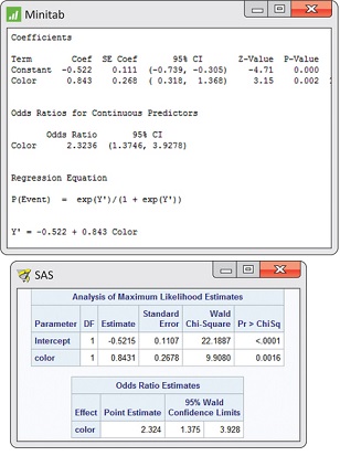
We conclude, “Servers wearing red are more likely to be tipped than servers wearing a different color (odds ratio=2.324, 95% CI=1.375 to 3.928).”
It is standard to use 95% confidence intervals, and software often reports these intervals. A 95% confidence interval for the odds ratio also provides a test of the null hypothesis that the odds ratio is 1 at the 5% significance level. If the confidence interval does not include 1, we reject H0 and conclude that the odds for the two groups are different; if the interval does include 1, the data do not provide enough evidence to distinguish the groups in this way.
Apply Your Knowledge
Question 17.8
CASE 17.117.8 Read the output.
Examine the Minitab and SAS output in Figure 17.3. Create a table that reports the estimates of β0 and β1 with the standard errors. Also report the odds ratio with its 95% confidence interval as given in this output.
Question 17.9
17.9 Inference for energy drink commercials.
Use software to run a logistic regression analysis for the energy drink commercial data of Exercise 17.1. Summarize the results of the inference.
17.9
log(odds)=−0.14306+0.20472x. The odds ratio estimate is 1.227; the 95% confidence interval is (0.761, 1.979).
energy
Question 17.10
17.10 Inference for audio/visual sharing.
Use software to run the logistic regression analysis for the audio/visual sharing data of Exercise 17.2. Summarize the results of the inference.
Examples of logistic regression analyses
The following example is typical of many applications of logistic regression. It concerns a designed experiment with five different values for the explanatory variable.
EXAMPLE 17.8 Effectiveness of an Insecticide
insect
As part of a cost-effectiveness study, a wholesale florist company ran an experiment to examine how well the insecticide rotenone kills an aphid called Macrosiphoniella sanborni that feeds on the chrysanthemum plant.3 The explanatory variable is the concentration (in log of milligrams per liter) of the insecticide. About 50 aphids each were exposed to one of five concentrations. Each insect was either killed or not killed. Here are the data, along with the results of some calculations:
| Concentration x (log scale) |
Number of insects |
Number killed |
Proportion killed ˆp |
Log odds |
| 0.96 | 50 | 6 | 0.1200 | −1.9924 |
| 1.33 | 48 | 16 | 0.3333 | −0.6931 |
| 1.63 | 46 | 24 | 0.5217 | 0.0870 |
| 2.04 | 49 | 42 | 0.8571 | 1.7918 |
| 2.32 | 50 | 44 | 0.8800 | 1.9924 |
Because there are replications at each concentration, we can calculate the proportion killed and estimate the log odds of death at each concentration. The logistic model in this case assumes that the log odds are linearly related to log concentration. Least-squares regression of log odds on log concentration gives the fit illustrated in Figure 17.4. There is a clear linear relationship, which justifies our use of the logistic model. The logistic regression fit for the proportion killed appears in Figure 17.5. It is a transformed version of Figure 17.4 with the fit calculated using the logistic model rather than least squares.
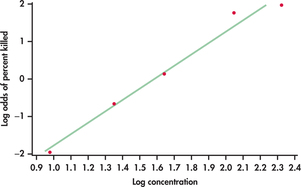
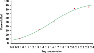
When the explanatory variable has several values, we can often use graphs like those in Figures 17.4 and 17.5 to visually assess whether the logistic regression model seems appropriate. Just as a scatterplot of y versus x in simple linear regression should show a linear pattern, a plot of log odds versus x in logistic regression should be close to linear. Just as in simple linear regression, outliers in the x direction should be avoided because they may overly influence the fitted model.
The graphs strongly suggest that insecticide concentration affects the kill rate in a way that fits the logistic regression model. Is the effect statistically significant? Suppose that rotenone has no ability to kill Macrosiphoniella san-borni. What is the chance that we would observe experimental results at least as convincing as what we observed if this supposition were true? The answer is the P-value for the test of the null hypothesis that the logistic regression slope is zero. If this P-value is not small, our graph may be misleading. As usual, we must add inference to our data analysis.
EXAMPLE 17.9 Does Concentration Affect the Kill Rate?
insect1
Figure 17.6 gives the output from JMP and Minitab for logistic regression analysis of the insecticide data. The model is
log(p1−p)=β0+β1x
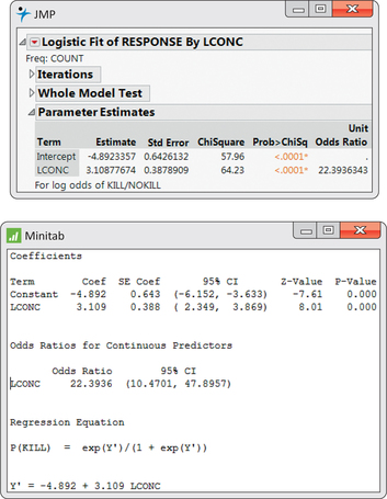
where the values of the explanatory variable x are 0.96, 1.33, 1.63, 2.04, 2.32. From the JMP output, we see that the fitted model is
log(odds)=b0+b1x=−4.8923+3.1088x
or
ˆp1−ˆp=e−4.8923+3.1088x
Figure 17.5 is a graph of the fitted ˆp given by this equation against x, along with the data used to fit the model. JMP gives the statistic X2 under the heading “ChiSquare.” The null hypothesis that β1=0 is clearly rejected (X2=64.23, P<0.0001).
The estimated odds ratio is 22.394. An increase of one unit in the log concentration of insecticide (x) is associated with a 22-fold increase in the odds that an insect will be killed. The confidence interval for the odds is given in the Minitab output: (10.470, 47.896).
Remember that the test of the null hypothesis that the slope is 0 is the same as the test of the null hypothesis that the odds ratio is 1. If we were reporting the results in terms of the odds, we could say, “The odds of killing an insect increase by a factor of 22.3 for each unit increase in the log concentration of insecticide (X2=64.23, P<0.0001; 95% CI=10.5 to 47.9).”
Apply Your Knowledge
Question 17.11
17.11 Find the 95% confidence interval for the slope.
Using the information in the output of Figure 17.6, find a 95% confidence interval for β1.
17.11
(2.349, 3.869).
Question 17.12
17.12 Find the 95% confidence interval for the odds ratio.
Using the estimate b1 and its standard error in the output of Figure 17.6, find the 95% confidence interval for the odds ratio and verify that this agrees with the interval given by Minitab.
Question 17.13
17.13 X2 or z.
The Minitab output in Figure 17.6 does not give the value of X2. The column labeled “Z-Value” provides similar information.
- Find the value under the heading “Z-Value” for the predictor LCONC. Verify that this value is simply the estimated coefficient divided by its standard error. This is a z statistic that has approximately the standard Normal distribution if the null hypothesis (slope 0) is true.
- Show that the square of z is X2. The two-sided P-value for z is the same as P for X2.
17.13
(a) Z=8.01. (b) 64.16, which agrees with the output up to rounding error.
In Example 17.6, we studied the problem of predicting whether a movie will be profitable using the log opening-weekend revenue as the explanatory variable. We now revisit this example to include the results of inference.
EXAMPLE 17.10 Predicting a Movie's Profitability
movprof
Figure 17.7 gives the output from Minitab for a logistic regression analysis using log opening-weekend revenue as the explanatory variable. The fitted model is
log(odds)=b0+b1x=−1.41+0.781x
This agrees up to rounding with the result reported in Example 17.6.
From the output, we see that because P=0.148, we cannot reject the null hypothesis that the slope β1=0. The value of the test statistic is z=1.45, calculated from the estimate b1=0.781 and its standard error SEb1=0.540. Minitab reports the odds ratio as 2.184, with a 95% confidence interval of (0.7584, 6.2898). Notice that this confidence interval contains the value 1, which is another way to assess H0:β1=0. In this case, we don't have enough evidence to conclude that this explanatory variable, by itself, is helpful in predicting the probability that a movie will be profitable.
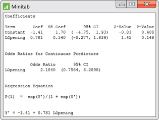
We estimate that a one-unit increase in the log opening-weekend revenue will increase the odds that the movie is profitable about 2.2 times. The data, however, do not give us a very accurate estimate. We do not have strong enough evidence to conclude that movies with higher opening-weekend revenues are more likely to be profitable. Establishing the true relationship accurately would require more data.