SECTION 5.3 Exercises
For Exercises 5.57 and 5.58, see page 276; and for 5.59, see page 278.
Question 5.60
5.60 What population and sample?
Twenty fourth-year students from your college who are majoring in English are randomly selected to be on a committee to evaluate changes in the statistics requirement for the major. There are 76 fourth-year English majors at your college. The current rules say that a statistics course is one of four options for a quantitative competency requirement. The proposed change would be to require a statistics course. Each of the committee members is asked to vote Yes or No on the new requirement.
- Describe the population for this setting.
- What is the sample?
- Describe the statistic and how it would be calculated.
- What is the population parameter?
- Write a short summary based on your answers to parts (a) through (d) using this setting to explain population, sample, parameter, statistic, and the relationships among these items.
Question 5.61
5.61 Simulating Poisson counts.
Most statistical software packages can randomly generate Poisson counts for a given μ. In this exercise, you will generate 1000 Poisson counts for μ=9.
- JMP users: With a new data table, right-click on header of Column 1 and choose Column Info. In the drag down dialog box named Column Properties, pick the Formula option. You will then encounter a Formula dialog box. Find and click in the Random Poisson function into the dialog box. Proceed to give the mean value of 9, which JMP refers to as “lambda.” Click OK twice to return to the data table. Finally, right-click on any cell of the column holding the formula, and choose the option of Add Rows. Input a value of 1000 for the number of rows to create and click OK. You will find 1000 random Poisson counts generated.
- Minitab users: Calc → Random Data → Poisson. Enter 1000 in the Number of row of data to generate dialog box, type “c1” in the Store in column(s) dialog box, and enter 9 in the Mean dialog box. Click OK to find the random Poisson counts in column c1.
- Produce a histogram of the randomly generated Poisson counts, and describe its shape.
- What is the sample mean of the 1000 counts? How close is this simulation estimate to the parameter value?
- What is the sample standard deviation of the 1000 counts? How close is this simulation estimate to the theoretical standard deviation?
5.61
Software, answers will vary. (a) The shape should be roughly symmetric. (b) The mean should be close to 9. (c) The standard deviation should be close to √9=3.
Question 5.62
5.62 Simulate a sampling distribution for ˆp.
In the previous exercise, you were asked to use statistical software’s capability to generate Poisson counts. Here, you will use software to generate binomial counts from the B(n, p) distribution. We can use this fact to simulate the sampling distribution for ˆp. In this exercise, you will generate 1000 sample proportions for p=0.70 and n=100.
- JMP users: With a new data table, right-click on header of Column 1 and choose Column Info. In the drag-down dialog box named Column Properties, pick the Formula option. You will then encounter a Formula dialog box. Find and click in the Random Binomial function into the dialog box. Proceed to give the values of 100 for n and 0.7 for p. Thereafter, click the division symbol found the calculator pad, and divide the binomial function by 100. Click OK twice to return to the data table. Finally, right-click on any cell of the column holding the formula, and choose the option of Add Rows. Input a value of 1000 for the number of rows to create and click OK. You will find 1000 sample proportions generated.
- Minitab users: Calc → Random Data → Binomial. Enter 1000 in the Number of row of data to generate dialog box, type “c1” in the Store in column(s) dialog box, enter 100 in the Number of trials dialog box, and enter 0.7 in the Event probability dialog box. Click OK to find the random binomial counts in column c1. Now use Calculator to define another column as the binomial counts divided by 100.
- Produce a histogram of the randomly generated sample proportions, and describe its shape.
- What is the sample mean of the 1000 proportions? How close is this simulation estimate to the parameter value?
- What is the sample standard deviation of the 1000 proportions? How close is this simulation estimate to the theoretical standard deviation?
Question 5.63
5.63 Simulate a sampling distribution.
In Exercise 1.72 (page 41) and Example 4.26 (pages 213–214), you examined the density curve for a uniform distribution ranging from 0 to 1. The population mean for this uniform distribution is 0.5 and the population variance is 1/12. Let’s simulate taking samples of size 2 from this distribution.
Use the RAND() function in Excel or similar software to generate 100 samples from this distribution. Put these in the first column. Generate another 100 samples from this distribution, and put these in the second column. Calculate the mean of the entries in the first and second columns, and put these in the third column. Now, you have 100 samples of the mean of two uniform variables (in the third column of your spreadsheet).
- Examine the distribution of the means of samples of size two from the uniform distribution using your simulation of 100 samples. Using the graphical and numerical summaries that you learned in Chapter 1, describe the shape, center, and spread of this distribution.
- The theoretical mean for this sampling distribution is the mean of the population that we sample from. How close is your simulation estimate to this parameter value?
- The theoretical standard deviation for this sampling distribution is the square root of 1/24. How close is your simulation estimate to this parameter value?
5.63
Software, answers will vary. (a) The shape should be roughly Normal. (b) The mean should be close to 0.5. (c) The standard deviation should be close to √1/24=0.2041.
Question 5.64
5.64 What is the effect of increasing the number of simulations?
Refer to the previous exercise. Increase the number of simulations from 100 to 500. Compare your results with those you found in the previous exercise. Write a report summarizing your findings. Include a comparison with the results from the previous exercise and a recommendation regarding whether or not a larger number of simulations is needed to answer the questions that we have regarding this sampling distribution.
Question 5.65
5.65 Change the sample size to 12.
Refer to Exercise 5.63. Change the sample size to 12 and answer parts (a) through (c) of that exercise. Note that the theoretical mean of the sampling distribution is still 0.5 but the standard deviation is the square root of 1/144 or, simply, 1/12. Investigate how close your simulation estimates are to these theoretical values. In general, explain the effect of increasing the sample size from two to 12 using the results from Exercise 5.63 and what you have found in this exercise.
5.65
Software, answers will vary. The distribution should be more Normal, the mean should be potentially closer to 0.5, but the spread will have decreased to 1/12=0.0833.
Question 5.66
5.66 Increase the number of simulations.
Refer to the previous exercise and to Exercise 5.64. Use 500 simulations to study the sampling distribution of the mean of a sample of size 12 from a uniform distribution. Write a summary of what you have found.
Question 5.67
5.67 Normal distributions.
Many software packages generate standard Normal variables by taking the sum of 12 uniform variables and subtracting 6.
- Simulate 1000 random values using this method.
- Use numerical and graphical summaries to assess how well the distribution of the 1000 values approximates the standard Normal distribution.
- Write a short summary of your work. Include details of your simulation.
5.67
Software, answers will vary. The distribution should look Normal. The mean should be close to 0, and the standard deviation should be close to 1.
Question 5.68
5.68 Is it unbiased?
A statistic has a sampling distribution that is somewhat skewed. The median is 5 and the quartiles are 2 and 10. The mean is 8.
- If the population parameter is 5, is the estimator unbiased?
- If the population parameter is 10, is the estimator unbiased?
- If the population parameter is 8, is the estimator unbiased?
- Write a short summary of your results in parts (a) through (c) and include a discussion of bias and unbiased estimators.
Question 5.69
5.69 The effect of the sample size.
Refer to Exercise 5.63, where you simulated the sampling distribution of the mean of two uniform variables, and Exercise 5.65, where you simulated the sampling distribution of the mean of 12 uniform variables.
- Based on what you know about the effect of the sample size on the sampling distribution, which simulation should have the smaller variability?
- Did your simulations confirm your answer in part (a)? Write a short paragraph about the effect of the sample size on the variability of a sampling distribution using these simulations to illustrate the basic idea. Be sure to include how you assessed the variability of the sampling distributions.
5.69
(a) The simulated mean using 12 uniform variables should have smaller variability than the simulated mean using only 2 uniform variables. (b) The simulations should have confirmed this.
Question 5.70
5.70 What’s wrong?
State what is wrong in each of the following scenarios.
- A parameter describes a sample.
- Bias and variability are two names for the same thing.
- Large samples are always better than small samples.
- A sampling distribution is something generated by a computer.
Question 5.71
5.71 Describe the population and the sample.
For each of the following situations, describe the population and the sample.
- A survey of 17,096 students in U.S. four-year colleges reported that 19.4% were binge drinkers.
- In a study of work stress, 100 restaurant workers were asked about the impact of work stress on their personal lives.
- A tract of forest has 584 longleaf pine trees. The diameters of 40 of these trees were measured.
5.71
(a) The population is all students in the United States at four-year colleges. The sample is the 17,096 people surveyed. (b) The population is all restaurant workers. The sample is the 100 people asked. (c) The population all 584 longleaf pine trees. The sample is the 40 trees measured.
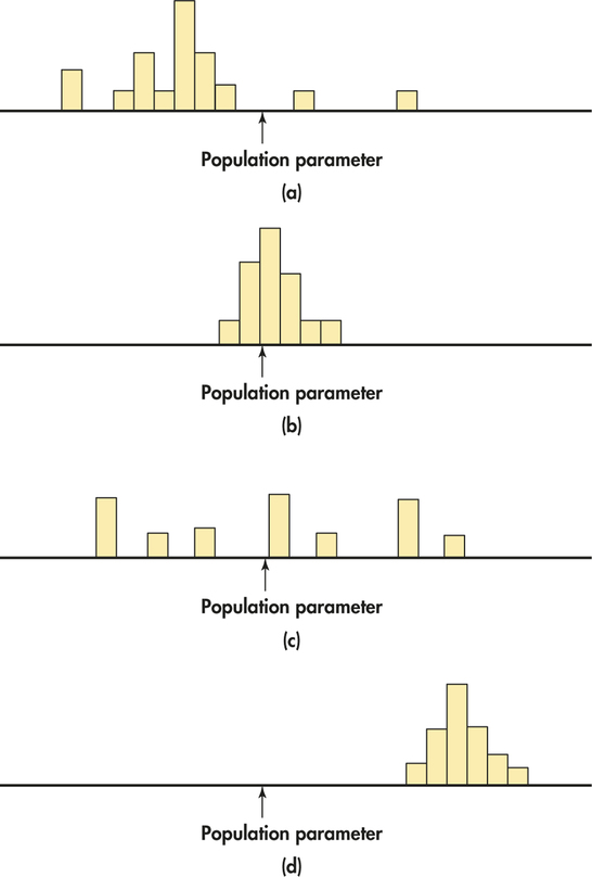
Question 5.72
5.72 Bias and variability.
Figure 5.15 shows histograms of four sampling distributions of statistics intended to estimate the same parameter. Label each distribution relative to the others as high or low bias and as high or low variability.