6.5 Power and Inference as a Decision
Although we prefer to use P-values rather than the reject-or-not view of the level α significance test, the latter view is very important for planning studies and for understanding statistical decision theory. We discuss these two topics in this section.
Power
Level α significance tests are closely related to confidence intervals—in fact, we saw that a two-sided test can be carried out directly from a confidence interval. The significance level, like the confidence level, says how reliable the method is in repeated use. If we use 5% significance tests repeatedly when H0 is, in fact, true, we will be wrong (the test will reject H0) 5% of the time and right (the test will fail to reject H0) 95% of the time.
The ability of a test to detect that H0 is false is measured by the probability that the test will reject H0 when an alternative is true. The higher this probability is, the more sensitive the test is.
Power
The probability that a level α significance test will reject H0 when a particular alternative value of the parameter is true is called the power of the test to detect that alternative.
EXAMPLE 6.26 The Power to Detect Departure from Target
CASE 6.1 Case 6.1 considered the following competing hypotheses:
H0:μ=473Ha:μ≠473
In Example 6.13 (page 317), we learned that σ=2 ml for the filling process. Suppose that the bottler Bestea wishes to conduct tests of the filling process mean at a 1% level of significance. Assume, as in Example 6.13, that 20 bottles are randomly chosen for inspection. Bestea’s operations personnel wish to detect a 1-ml change in mean fill amount, either in terms of underfilling or overfilling. Does a sample of 20 bottles provide sufficient power?
We answer this question by calculating the power of the significance test that will be used to evaluate the data to be collected. Power calculations consist of three steps:
- State H0, Ha (the particular alternative we want to detect), and the significance levelα.
- Find the values of ˉx that will lead us to reject H0.
- Calculate the probability of observing these values of ˉx when the alternative is true.
Let’s go through these three steps for Example 6.26.
Step 1. The null hypothesis is that the mean filling amount is at the 473-ml target level. The alternative is two-sided in that we wish to detect change in either direction from the target level. Formally, we have
H0:μ=473Ha:μ≠473
In the possible values of the alternative, we are particularly interested in values at a minimal 1 ml from 472. This would mean that we are focusing on μ values of 472 or 474. We can proceed with the power calculations using either one of these values. Let’s pick the specific alternative of μ=472.
Step 2. The test statistic is
z=ˉx−4732/√20
From Table D, we find that z-values less than −2.576 or greater than 2.576 would be viewed as signifcant at the 1% level. Consider first rejection above 2.576. We can rewrite the upper rejection rule in terms of ˉx:
ˉx−4732/√20≥2.576ˉx≥473+2.5762√20ˉx≥474.152
We can do the same sort of rearrangement with the lower rejection rule to find rejection is also associated with:
ˉx≤471.848
Step 3. The power to detect the alternative μ=472 is the probability that H0 will be rejected when, in fact, μ=472. We calculate this probability by standardizing ˉx using the value μ=472, the population standard deviation σ=2, and the sample size n=20. We have to remember that rejection can happen when either ˉx≤471.848 or ˉx≥474.152 These are disjoint events, so the power is the sum of their probabilities, computed assuming that the alternative μ=472 is true. We find that
P(ˉx≥474.152)=P(ˉx−μσ/√n≥474.152−4722/√20)=P(Z≥4.81)˙=0P(ˉx≤471.848)=P(ˉx−μσ/√n≤471.848−4722/√20)=P(Z≤−0.340)=0.37
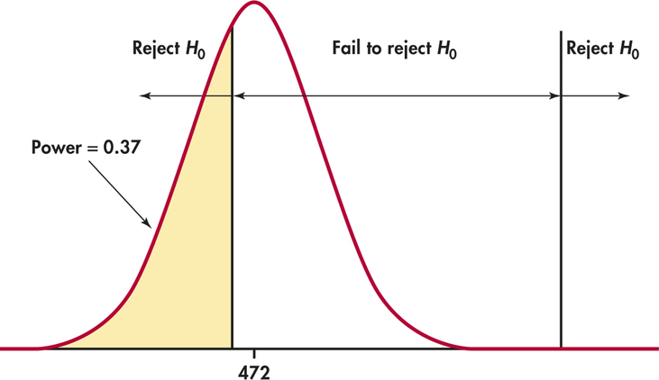
Figure 6.18 illustrates this calculation. Because the power is only about 0.37, we are not strongly confident that the test will reject H0 when this alternative is true.
Increasing the power
Suppose that you have performed a power calculation and found that the power is too small. What can you do to increase it? Here are four ways:
- Increase α. A 5% test of significance will have a greater chance of rejecting the alternative than a 1% test because the strength of evidence required for rejection is less.
- Consider a particular alternative that is farther away from μ0.Values of μ that are in Ha but lie close to the hypothesized value μ0 are harder to detect (lower power) than values of μ that are far from μ0.
- Increase the sample size. More data will provide more information about ˉx so we have a better chance of distinguishing values of μ.
- Decrease σ. This has the same effect as increasing the sample size: more information about μ. Improving the measurement process and restricting attention to a subpopulation are possible ways to decrease σ.
Power calculations are important in planning studies. Using a significance test with low power makes it unlikely that you will find a signifcant effect even if the truth is far from the null hypothesis. A null hypothesis that is, in fact, false can become widely believed if repeated attempts to find evidence against it fail because of low power.
In Example 6.26, we found the power to be 0.37 for the detection of a 1-ml departure from the null hypothesis. If this power is unsatisfactory to the bottler, one option noted earlier is to increase the sample size. Just how large should the sample be? The following example explores this question.
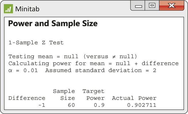
EXAMPLE 6.27 Choosing Sample Size for a Desired Power
CASE 6.1 Suppose the bottler Bestea desires a power of 0.9 in the detection of the specific alternative of μ=472. From Example 6.26, we found that a sample size of 20 offers a power of only 0.37. Manually, we can repeat the calculations found in Example 6.26 for different values of n larger than 20 until we find the smallest sample size giving at least a power of 0.9. Fortunately, most statistical software saves us from such tedium. Figure 6.19 shows Minitab output with inputs of 0.9 for power, 1% for sig-nifcance level, 2 for σ, and -1(=472-473) for the departure amount from the null hypothesis. From the output, we learn that a sample size of at least 60 is needed to have a power of at least 0.9. If we used a sample size of 59, the actual power would be a bit less than the target power of 0.9.
Inference as decision
We have presented tests of significance as methods for assessing the strength of evidence against the null hypothesis. This assessment is made by the P-value, which is a probability computed under the assumption that H0 is true. The alternative hypothesis (the statement we seek evidence for) enters the test only to help us see what outcomes count against the null hypothesis.
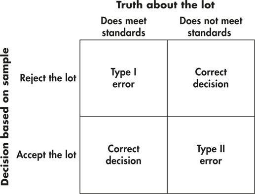
There is another way to think about these issues. Sometimes, we are really concerned about making a decision or choosing an action based on our evaluation of the data. The quality control application of Case 6.1 is one circumstance. In that application, the bottler needs to decide whether or not to make adjustments to the filling process based on a sample outcome. Consider another example. A producer of ball bearings and the consumer of the ball bearings agree that each shipment of bearings shall meet certain quality standards. When a shipment arrives, the consumer inspects a random sample of bearings from the thousands of bearings found in the shipment. On the basis of the sample outcome, the consumer either accepts or rejects the shipment. Let’s examine how the idea of inference as a decision changes the reasoning used in tests of significance.
Two types of error
Tests of significance concentrate on H0, the null hypothesis. If a decision is called for, however, there is no reason to single out H0. There are simply two hypotheses, and we must accept one and reject the other. It is convenient to call the two hypotheses H0 and Ha, but H0 no longer has the special status (the statement we try to find evidence against) that it had in tests of significance. In the ball bearing problem, we must decide between
H0:the shipment of bearings meets standardsHa:the shipment does not meet standards
on the basis of a sample of bearings.
We hope that our decision will be correct, but sometimes it will be wrong. There are two types of incorrect decisions. We can accept a bad shipment of bearings, or we can reject a good shipment. Accepting a bad shipment leads to a variety of costs to the consumer (for example, machine breakdown due to faulty bearings or injury to end-product users such as skateboarders or bikers), while rejecting a good shipment hurts the producer. To help distinguish these two types of error, we give them specific names.
Type I and Type II Errors
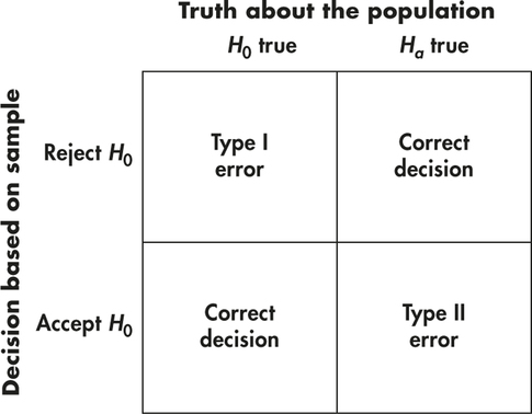
If we reject H0 (accept Ha) when in fact H0 is true, this is a Type I error.
If we accept H0 (reject Ha) when in fact Ha is true, this is a Type II error.
The possibilities are summed up in Figure 6.20. If H0 is true, our decision either is correct (if we accept H0) or is a Type I error. If Ha is true, our decision either is correct or is a Type II error. Only one error is possible at one time. Figure 6.21 applies these ideas to the ball bearing example.
Error probabilities
We can assess any rule for making decisions in terms of the probabilities of the two types of error. This is in keeping with the idea that statistical inference is based on probability. We cannot (short of inspecting the whole shipment) guarantee that good shipments of bearings will never be rejected and bad shipments will never be accepted. But by random sampling and the laws of probability, we can say what the probabilities of both kinds of error are.
Significance tests with fixed level α give a rule for making decisions because the test either rejects H0 or fails to reject it. If we adopt the decision-making way of thought, failing to reject H0 means deciding to act as if H0 is true. We can then describe the performance of a test by the probabilities of Type I and Type II errors.
EXAMPLE 6.28 Diameters of Bearings
The diameter of a particular precision ball bearing has a target value of 20 millimeters (mm) with tolerance limits of ±0.001 mm around the target. Suppose that the bearing diameters vary Normally with standard deviation of sixty-five hundred-thousandths of a millimeter, that is, σ=0.00065 mm. When a shipment of the bearings arrives, the consumer takes an SRS of five bearings from the shipment and measures their diameters. The consumer rejects the bearings if the sample mean diameter is signif-cantly different from 20 mm at the 5% significance level.
This is a test of the hypotheses
H0:μ=20Ha:μ≠20
To carry out the test, the consumer computes the z statistic:
z=ˉx−200.00065/√5
and rejects H0 if
z<−1.96orz>1.96
A Type I error is to reject H0 when in fact μ=20.
What about Type II errors? Because there are many values of μ in Ha, we concentrate on one value. Based on the tolerance limits, the producer agrees that if there is evidence that the mean of ball bearings in the lot is 0.001 mm away from the desired mean of 20 mm, then the whole shipment should be rejected. So, a particular Type II error is to accept H0 when in fact μ=20+0.001=20.001.
Figure 6.22 shows how the two probabilities of error are obtained from the two sampling distributions of ˉx, for μ=20 and for μ=20.001. When μ=20, H0 is true and to reject H0 is a Type I error. When μ=20.001, accepting H0 is a Type II error. We will now calculate these error probabilities.
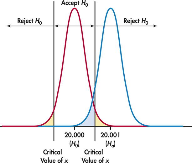
The probability of a Type I error is the probability of rejecting H0 when it is really true. In Example 6.28, this is the probability that |z|≥1.96 when μ=20. But this is exactly the significance level of the test. The critical value 1.96 was chosen to make this probability 0.05, so we do not have to compute it again. The definition of “signifcant at level 0.05” is that sample outcomes this extreme will occur with probability 0.05 when H0 is true.
Significance and Type I Error
The significance level α of any fixed level test is the probability of a Type I error. That is, α is the probability that the test will reject the null hypothesis H0 when H0 is in fact true.
The probability of a Type II error for the particular alternative μ=20.001 in Example 6.28 is the probability that the test will fail to reject H0 when μ has this alternative value. The power of the test for the alternative μ=20.001 is just the probability that the test does reject H0 when Ha is true. By following the method of Example 6.26, we can calculate that the power is about 0.93. Therefore, the probability of a Type II error is equal to 1−0.93, or 0.07. It would also be the case that the probability of a Type II error is 0.07 if the value of the alternative μ is 19.999, that is, 0.001 less than the null hypothesis mean of 20.
Power and Type II Error
The power of a fixed level test for a particular alternative is 1 minus the probability of a Type II error for that alternative.
The two types of error and their probabilities give another interpretation of the significance level and power of a test. The distinction between tests of significance and tests as rules for deciding between two hypotheses lies, not in the calculations but in the reasoning that motivates the calculations. In a test of significance, we focus on a single hypothesis (H0) and a single probability (the P-value). The goal is to measure the strength of the sample evidence against H0. Calculations of power are done to check the sensitivity of the test. If we cannot reject H0, we conclude only that there is not sufficient evidence against H0, not that H0 is actually true. If the same inference problem is thought of as a decision problem, we focus on two hypotheses and give a rule for deciding between them based on the sample evidence. We must therefore, focus equally on two probabilities—the probabilities of the two types of error. We must choose one or the other hypothesis and cannot abstain on grounds of insufficient evidence.
The common practice of testing hypotheses
Such a clear distinction between the two ways of thinking is helpful for understanding. In practice, the two approaches often merge. We continued to call one of the hypotheses in a decision problem H0. The common practice of testing hypotheses mixes the reasoning of significance tests and decision rules as follows:
- State H0 and Ha just as in a test of significance.
- Think of the problem as a decision problem so that the probabilities of Type I and Type II errors are relevant.Page 350
- Because of Step 1, Type I errors are more serious. So choose an α (significance level) and consider only tests with probability of a Type I error no greater thanα.
- Among these tests, select one that makes the probability of a Type II error as small as possible (that is, power as large as possible). If this probability is too large, you will have to take a larger sample to reduce the chance of an error.
Testing hypotheses may seem to be a hybrid approach. It was, historically, the effective beginning of decision-oriented ideas in statistics. An impressive mathematical theory of hypothesis testing was developed between 1928 and 1938 by Jerzy Neyman and Egon Pearson. The decision-making approach came later (1940s). Because decision theory in its pure form leaves you with two error probabilities and no simple rule on how to balance them, it has been used less often than either tests of significance or tests of hypotheses. Decision ideas have been applied in testing problems mainly by way of the Neyman-Pearson hypothesis-testing theory. That theory asks you first to chooseα, and the influence of Fisher has often led users of hypothesis testing comfortably back to α=0.05 or α=0.01. Fisher, who was exceedingly argumentative, violently attacked the Neyman-Pearson decision-oriented ideas, and the argument still continues.