Example 2.16

EXAMPLE 2.16 Education Spending and Population

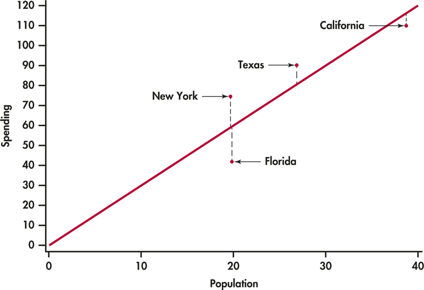
CASE 2.1 Figure 2.13 is a scatterplot showing education spending versus the population for the 50 states that we studied in Case 2.1 (page 65). Included on the scatterplot is the least-squares line. The points for the states with large values for both variables—California, Texas, Florida, and New York—are marked individually.

The equation of the least-squares line is where represents education spending and x represents the population of the state.

Let’s look carefully at the data for California, y = 110.1 and x = 38.7. The predicted education spending for a state with 38.7 million people is

The residual for California is the difference between the observed spending (y) and this predicted value.

Figure 2.13: FIGURE 2.13 Scatterplot of spending on education versus the population for 50 states, with the least-squares line and selected points labeled, Example 2.16.