The distribution properties of populations can be estimated

Although we can easily define the distribution properties of populations, how do we actually quantify them? Four of the properties—abundance, density, geographic range, and dispersion—require that we determine where individuals are located and how many are located in particular areas. The fifth property, dispersal, is somewhat unique because it requires that we quantify the movement of individuals.

Quantifying the Location and Number of Individuals

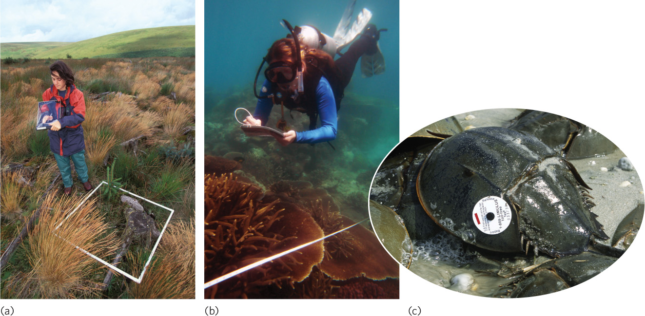
One way to determine the number of individuals in an area is to conduct a census, which means counting every individual in a population. Every 10 years, for example, the United States government attempts a census with the goal of counting every person living in the country. For most species, however, it is not feasible to count every individual in the population. As a result, scientists must conduct a survey, in which they count a subset of the population. Using these samples, they estimate the abundance, density, and distribution of the population. Scientists have developed a variety of ways to make these estimates, including area- and volume-based surveys, line-transect surveys, and mark-recapture surveys (Figure 11.8).

Figure 11.8 Estimating population abundance, density, and distribution. (a) Area-based studies count the number of individuals within a fixed area, such as this researcher working on the Dendles National Natural Reserve in England. (b) Linear-transect studies, including this one at the Great Barrier Reef in Australia, count the number of individuals that are observed along a predefined line. (c) Mark-recapture studies collect a sample of the population, mark them, and then return them. For example, horseshoe crabs (Limulus polyphemus) in Delaware are marked with small circular tags. A short time later, a second sample is collected to determine the proportion of marked animals in the population, which can be used to estimate the size of the total population.

Photos by (a) Paul Glendell/Alamy; (b) Suzanne Long/Alamy; (c) Patrick W. Grace/Photo Researchers, Inc.

Area- and Volume-Based Surveys

Area- and volume-based surveys define the boundaries of an area or volume and then count all of the individuals within that space. The size of the defined space is typically related to the abundance and density of the population. For example, researchers who wish to know the number of bacteria in the soil might collect samples of soil that are only a few cubic centimeters in volume. In contrast, researchers who wish to know the number of individual corals on a coral reef might sample areas that are 1 m². At the most extreme, researchers who want to estimate the abundance, density, and distribution of large mammals might count the number of individuals in aerial photos that cover hundreds of square meters. By taking multiple samples, scientists can determine how many individuals are present in an average sample area of land or volume of soil or water.

Line-Transect Surveys

Line-transect surveys count the number of individuals observed as one moves along a line. There are many variations on this technique. For example, researchers examining small plants in a field or forest might tie a long string between two fixed points and count the number of individuals the string crosses. Alternatively, researchers might count all individuals that are observed within a fixed distance of a line, such as the number of trees on a savanna located within 100 m of a line. A similar approach has been used in surveys of amphibians. In this case, observers count the number of frogs that can be heard along a predetermined path. If we know how far, on average, a person can hear a frog call, we can estimate the number of frogs calling in an area that includes both sides of the path. Such line-transect data can be converted into area estimates.

One of the most famous line-transect studies is the annual Christmas bird count. The bird count began in 1900 when 27 volunteers from the Audubon Society positioned themselves at different locations in North America and counted all the birds they saw in one day. Today, tens of thousands of volunteers go outside during their winter holidays and follow a predetermined path that covers a 24-km circle. Throughout the day, the volunteers count the number of individuals of every bird species they can see or hear within this circle. This long-term survey of birds in North America has provided incredibly valuable data that has helped scientists determine which species of birds have populations that are increasing, stable, or declining.

Mark-Recapture Surveys

Area- and volume-based and line-transect studies are very useful for organisms that do not move—such as plants and corals—or animals that are not easily disturbed—such as snails—and therefore less likely to leave the area while a location is being sampled. Some animals, however, are very sensitive to the presence of researchers and will leave the area while other species are well camouflaged and difficult to find. Both situations can cause us to underestimate the number of individuals in a population, so for these situations we need a different type of sampling technique. One effective method is the use of mark-recapture surveys. As the name implies, mark-recapture surveys collect a number of individuals from a population and mark them. These individuals are then returned to the population. Once enough time has passed for the marked individuals to mingle throughout the population, a second sample of the population is made. Based on the number originally marked, the total number collected the second time, and the number of marked animals collected the second time, we can estimate the size of the population. Mark-recapture studies are commonly conducted on birds, fish, mammals, and highly mobile invertebrates. The actual calculations for arriving at this estimate are discussed below in “Analyzing Ecology: Mark-Recapture Surveys.”

Quantifying the Dispersal of Individuals

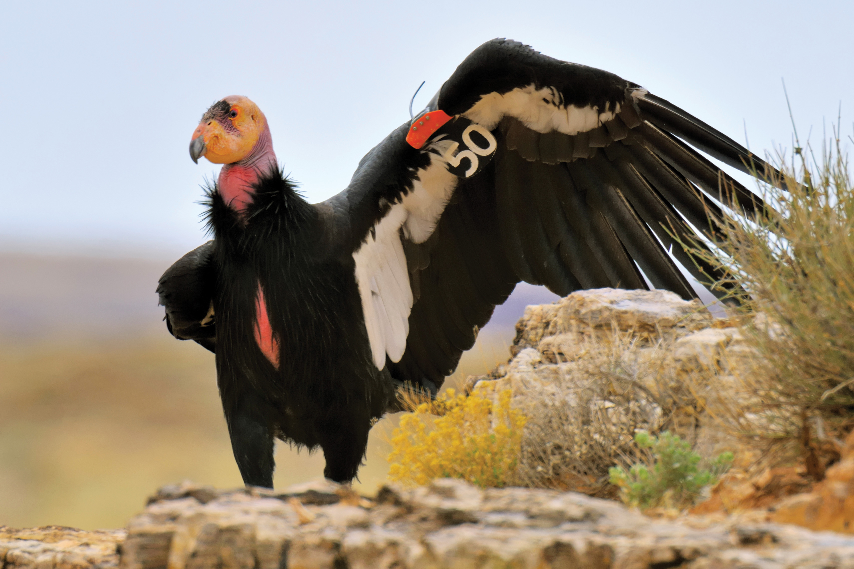
Quantifying the dispersal of individuals from a population requires identifying the source of individuals. As we will see, this can be done by ensuring that there is only one possible source of individuals and then determining how far individuals disperse from this single location. In other cases, individuals are marked and then observed or recaptured at some later time to determine how far they moved from the location where they were marked (Figure 11.9). In animal studies, possible marks include ear tags, radio transmitters, or leg bands. In plant studies, researchers can mark pollen with fluorescent powders and then examine surrounding flowers to determine how far the pollen grains have been moved either by the wind or by pollinators.

Figure 11.9 Measuring dispersal. This California condor (Gymnogyps californianus), which was captured in the Grand Canyon National Park in Arizona, has been marked using a wing band that has a unique number to identify where it hatched and how far it dispersed.

Photo by Thomas & Pat Leeson/Photo Researchers, Inc.

A common measure of dispersal is the lifetime dispersal distance, which is the average distance that an individual moves from where it was hatched or born to where it reproduces. By knowing the lifetime dispersal distance, we can also estimate how rapidly a growing population can increase its geographic range. For example, when researchers marked eight species of songbirds with leg bands, they found that lifetime dispersal distances averaged between 344 and 1,681 m. A lifetime dispersal distance of about 1 km per generation is therefore not unusual for populations of songbirds. At this rate, the descendants of an average individual might traverse an entire continent in a thousand generations or so.

These calculations suggest that it will take an average species of songbird more than 1,000 generations of dispersal to travel across a continent. However, it can actually happen much faster because a few individuals in a population can disperse much farther than the average bird in the population. An excellent example of this occurred following the introduction of the European starling to the United States. In 1890 and 1891, 160 European starlings were released in the vicinity of New York City. Within 60 years, the population had spread 4,000 km from New York to California, at an average rate of about 67 km per year. You can see this rapid spread of starlings in Figure 11.10. The expansion occurred rapidly because a few individuals dispersed much longer distances than the average, and established new populations beyond the range boundary of the species. Although the few individuals that might move over such long distances are rare, they can have large effects on population distributions. Today, the starling lives throughout most of the United States.

Figure 11.10 The rapid dispersal of European starlings across the United States. After being introduced near New York City in 1890 and 1891, the bird rapidly spread across the United States over a 60-year period. The blue-shaded area represents the range of breeding populations. The blue dots indicate detections of starlings that exhibited unusually long dispersal, thereby facilitating the rapid spread of the species. Today, the starling population covers more than 7 million km² of North America from coast to coast.

Data from B. Kessel, Distribution and migration of the European starling in North America, Condor 55 (1953): 49–67; and the U.S. Geological Survey (2003), http://www.mbrpwrc.usgs.gov/bbs/htm03/ra2003_red/ra04930.htm