Many populations live in distinct patches of habitat

In our discussion of the collared lizard, we saw that individuals in the region live in many small groups, with each group restricted to a particular glade. The lizards also move between habitats, but such movement depends on the quality of the forested habitat connecting the glades. When ecologists want to understand the movement of individuals among patches of habitats and how this affects the abundance of animals in each patch of habitat, they need to consider the quality of the habitat. They also have to consider the difficulty in reaching the habitat, which is determined by the distance to the habitat and the difficulty in crossing the area between habitat patches. In this section, we will explore how habitat quality affects the distribution of individuals among habitats and how ecologists have conceptualized the distribution and movement of individuals among suitable patches of habitat.

The Ideal Free Distribution Among Habitats

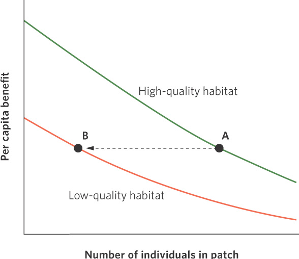
When habitats differ in quality and individuals can easily move among habitat patches, natural selection should favor those individuals that can choose the habitat that provides them with the most energy; this would improve their fitness. If all individuals are able to distinguish between high- and low-quality habitats, and assess the benefit of living in either habitat, then all individuals should initially move to the high-quality habitats, which are represented by a green line in Figure 11.16. However, as more and more individuals choose the high-quality habitat, the resources available must be divided among many individuals. This reduces the amount of resources available to each individual, also known as the per capita benefit. At some point, the per capita benefit in the high-quality habitat falls so low that an individual would be better off if it moved over to the low-quality habitat, which is indicated by the orange line in Figure 11.16. Continued increases in the population size would continue to add individuals to both the high- and low-quality habitats such that individuals in both habitats would experience the same per capita benefit. When all individuals have perfect knowledge of habitat variation and they distribute themselves in a way that allows them to have the same per capita benefit, we call it the ideal free distribution.

Figure 11.16 The ideal free distribution. Given the existence of high- and low-quality habitats, the first individual to arrive should select the high-quality habitat. As more individuals choose the high-quality habitat, however, the per capita benefit of the habitat declines. At some point (point A), it is equally beneficial for an individual to move to the low-quality habitat (point B) because the per capita benefit equals that experienced in the high-quality habitat. Although the low-quality habitat will have fewer individuals than the high-quality habitat, all individuals will experience the same per capita benefits.

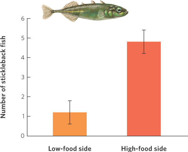
An example of individuals exhibiting an ideal free distribution can be seen in an experiment in which stickleback fish (Gasterosteus aculeatus) were presented with high- and low-quality habitats. Using water fleas (Daphnia magna), which are readily consumed by stickleback fish, the researchers added different numbers of water fleas to opposite ends of an aquarium so that each end of the aquarium represented a habitat of different quality. When the first fish were initially placed into the aquarium with no water fleas present, the fish were distributed equally between the two halves of the aquarium. In one experiment, researchers added 30 water fleas per minute to one end of an aquarium and six per minute to the other, a ratio of five to one. The results of this experiment are shown in Figure 11.17. Within 5 minutes, the fish had distributed themselves between the two halves in a ratio that was approximately four to one, which is close to the five to one ratio predicted by an ideal free distribution. When the provisioning ratio was changed—that is, the high- and low-quality patches were switched between ends of the aquarium—the fish quickly adjusted their distribution ratio. How they achieved this ideal free distribution was not determined, but they may have used the rate at which they encountered food items, or perhaps the number of other fish close by, as cues to patch quality.

Figure 11.17 The ideal free distribution in stickleback fish. When six fish were placed in an aquarium with the two ends receiving a five-to-one difference in food rations, the fish distributed themselves in a four-to-one ratio. As a result, each fish received a similar per capita amount of food. Error bars are standard deviations.

Data from M. Milinski, An evolutionarily stable feeding strategy in sticklebacks, Zeitschrift für Tierpsychologie 51 (1979): 36–40.

The ideal free distribution tells us how individuals should distribute themselves among habitats of differing quality, but individuals in nature rarely match the ideal expectations. In some cases individuals may not be aware that other habitats exist. Also, the fitness of an individual is not solely determined by maximizing its resources. Other factors that influence an individual’s use of a particular habitat include the presence of predators or of a territory owner that precludes moving into a high-quality habitat.

When reproductive success has been measured in the field, ecologists commonly find that individuals living in high-quality habitats have higher reproductive success. Often dominant individuals have monopolized the best resources, and they tend to produce surplus offspring while individuals in the poorest habitats do not produce enough offspring to replace themselves. As a result, the populations living in the high-quality habitats serve as a source of dispersing offspring that move to low-quality habitats, which allows populations in low-quality habitats to persist.

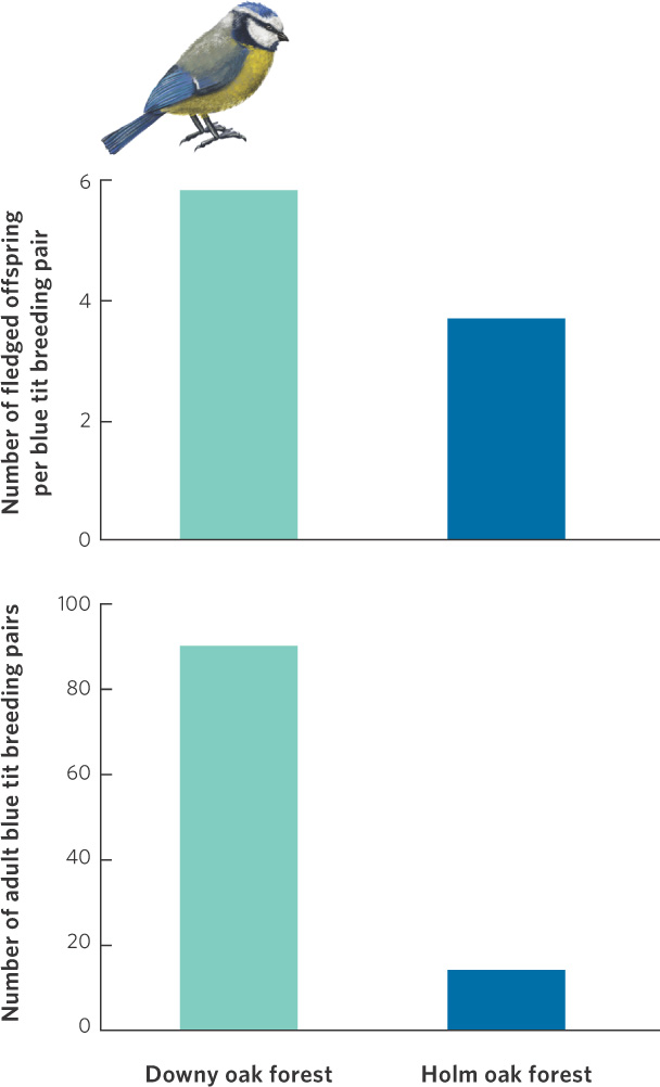
A study of the blue tit (Parus caeruleus), a small songbird from southern Europe, helps to illustrate this point. The blue tit breeds in two kinds of forest habitat, one dominated by the deciduous downy oak (Quercus pubescens) and the other by the evergreen holm oak (Quercus ilex). Long-term studies in southern France have revealed that the downy oak habitat produces more caterpillars, an important food item for the blue tits. This difference in caterpillar availability is reflected in the population densities of the birds. As you can see in Figure 11.18, the downy oak forest supports more than six times as many adult breeding pairs as the holm oak forest. Moreover, each breeding pair produces about 60 percent more offspring per year in the downy oak forest than in the holm oak forest. If we assume that juvenile survival is 20 percent in the first year and that annual adult survival is 50 percent—values that are typical of temperate songbirds— the population in the downy oak habitat would experience an annual growth of 9 percent per year if the surplus individuals did not disperse out of the habitat. At the same time, the population in the low-quality, holm oak habitat would experience an annual decline of 13 percent per year if no birds emigrated from the high-quality habitat. This would cause the population in the low-quality habitat to rapidly go extinct. In reality, the populations persist over time because the low-quality habitat receives surplus individuals from the high-quality habitat.

Figure 11.18 The effects of habitat quality. In blue tit songbirds, deciduous downy oak forests support many more adult breeding pairs than evergreen holm oak forests. In addition, birds living in the downy oak forest produce about 60 percent more fledglings per nest.

Data from J. Blondel, Habitat heterogeneity and life-history variation of Mediterranean blue tits (Parus caeruleus), The Auk 110 (1993): 511–520.

Conceptual Models of Spatial Structure

The ideal free distribution examines how individuals should distribute themselves when they know about the quality of different habitats and can freely move among them. In many cases, however, it is not easy to move from one patch of habitat to another, either because the other patches are relatively far away or because the region between the patches is fairly inhospitable. In such scenarios, most individuals in the patch stay put, only occasionally dispersing to other habitat patches. As a result, the larger population is broken up into smaller groups of conspecifics that live in isolated patches, which we call subpopulations.

When individuals frequently disperse among subpopulations, the whole population functions as a single structure and they all increase and decrease in abundance synchronously. When dispersal is infrequent, however, the abundance of individuals in each subpopulation can fluctuate independently of one another. In considering the spatial structure of subpopulations, ecologists have devised three models: the basic metapopulation model, the source–sink metapopulation model, and the landscape metapopulation model. These three models range from less to more complex. We shall explore the dynamics of these models in more detail in Chapter 12.

The Basic Metapopulation Model

The basic metapopulation model describes a scenario in which there are patches of suitable habitat embedded within a matrix of unsuitable habitat. All suitable patches are assumed to be of equal quality. Some suitable patches are occupied while others are not, although the unoccupied patches can be colonized by dispersers from occupied patches. The basic metapopulation models emphasize how colonization and extinction events can affect the proportion of total suitable habitats that are occupied.

The Source–Sink Metapopulation Model

The source-sink metapopulation model builds upon the basic metapopulation model and adds the reality that different patches of suitable habitat are not of equal quality. As we saw in the study of blue tits, it is common that occupants of high-quality habitats serve as a source of dispersers. Such populations are referred to as source subpopulations. At the same time, there can be low-quality habitats that rarely produce enough surplus offspring to produce any dispersers. These habitats depend on outside dispersers to maintain the subpopulation. These subpopulations are known as sink subpopulations.

The Landscape Metapopulation Model

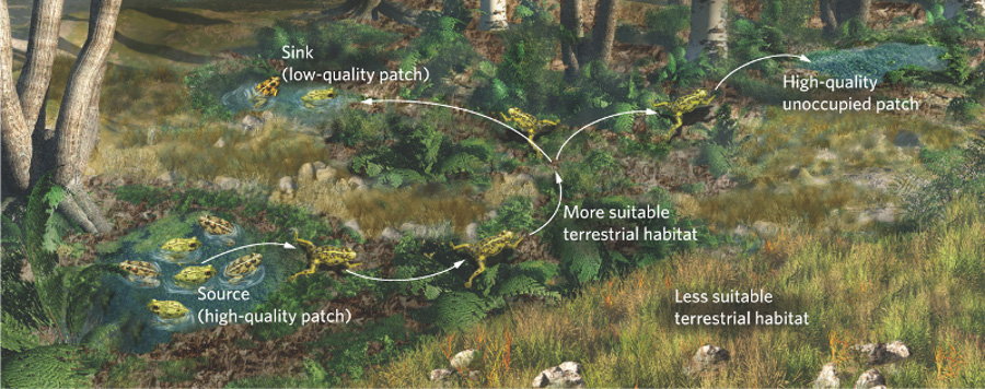
The landscape metapopulation model is even more realistic than the source–sink model because it considers both differences in the quality of the suitable patches and the quality of the surrounding matrix. As we discussed earlier in this chapter, the habitat in the surrounding matrix can vary in quality for dispersing organisms. Consider, for example, the challenge that metamorphosing frogs have when they move from their natal pond. They face risks of both predation and desiccation. Moving through a grassy field poses a much higher risk of predation and drying out than moving through a humid forest. Although neither field nor forest is a suitable habitat for the frog to reproduce, each presents different magnitudes of dispersal barriers. For a regional population of collared lizards to persist and grow requires both high-quality glade habitats and a high-quality matrix of open forest that facilitates dispersal. The landscape model, which is illustrated in Figure 11.19, represents the most realistic, yet also the most complex, spatial structure of populations.

Figure 11.19 The landscape metapopulation model. The landscape model contains the most realistic conditions of habitat patches that differ in quality and a surrounding matrix that is variable in its suitability for dispersal and the presence of dispersal barriers.

Throughout this chapter we have examined the spatial structure of populations by considering the characteristics of abundance, density, and geographic range. We have also focused on the importance of suitable habitats and dispersal and how ecological niche modeling can help us predict the distributions of populations in the future. In doing so, we have largely ignored the fact that populations increase and decrease in abundance, but in the next chapter, we will take an in-depth exploration of how populations grow and how this growth is regulated.

ECOLOGY TODAY CONNECTING THE CONCEPTS

THE INVASION OF THE EMERALD ASH BORER

The emerald ash borer. After being accidentally introduced to the United States in the 1990s, the insect has decimated ash tree populations.

Photo by David Cappaert, Michigan State University, Bugwood.org.

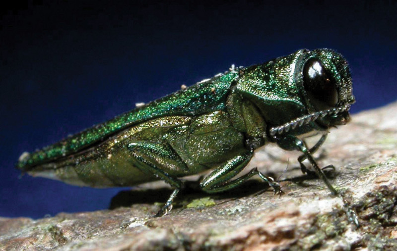
In 2002, a beautiful green insect, the emerald ash borer (Agrilus planipennis), was observed for the first time in North America. A native of eastern Asia, it had never lived in North America and was unfamiliar to most people. Over the next decade, its population grew and the emerald ash borer became one of the most numerous invasive pests on the continent.

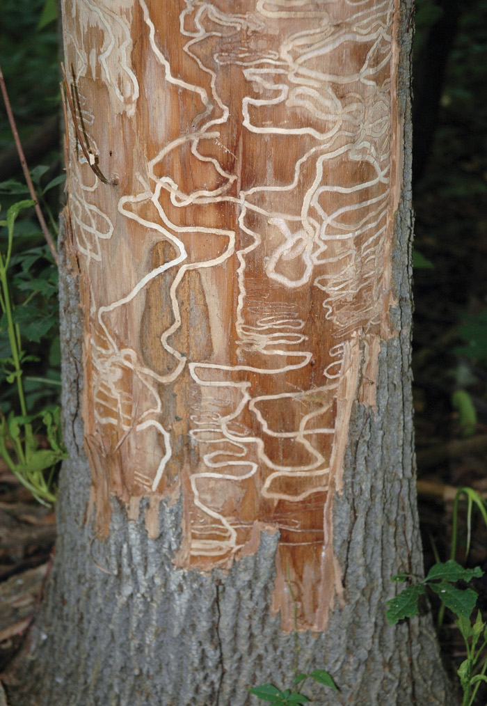
The expanse of inhospitable oceans had previously prevented the emerald ash borer from dispersing to North America. Researchers suspect that the insect arrived in the 1990s from Asia by accidentally hitching a ride inside wooden crates that were shipped from Asia to Detroit, Michigan. Once they arrived in Michigan, they found an abundant supply of their favorite food: ash trees. The adult insect does little harm to ash trees, but it lays eggs in the cracks of the tree’s bark. When the eggs hatch, the larvae live in clustered distributions and they consume the underlying cambium and phloem of the trees. Because the cambium is essential to tree growth and the phloem is essential for transporting nutrients, the consumption of this tissue by the larvae causes an ash tree to die within 2 to 3 years. Mature larvae metamorphose into adult beetles and the cycle starts all over again.

Midwestern forests have an abundance of ash trees, and the beetle population grew rapidly in just a few years. However, the beetle has a fairly short dispersal distance, rarely moving more than 100 m from where it first emerges as an adult, so one would expect the geographic range of this pest to expand slowly due to its dispersal limitation. But the beetle’s range expanded rapidly through unintentional human assistance. As ash trees were dying, many of them were cut down for firewood. Much of this firewood was carried long distances for events such as camping trips, which allowed the beetle to colonize new subpopulations. The impact of this assisted dispersal has been dramatic. In 2012, only 10 years since its discovery, the emerald ash borer already covered a range from Ontario and Quebec to Missouri and Tennessee and from Wisconsin and Iowa to Virginia and Pennsylvania. In all of these states and provinces, biologists have set up survey traps containing beetle sex attractants to estimate the abundance and density of beetles in the area.

268

American ash tree. The larvae of the emerald ash borer consume the underlying cambium and phloem under the bark of the trees, causing the trees to die.

Photo by Art Wagner, Washington State Department of Agriculture, Bugwood.org.

The emerald ash borer has already killed tens of millions of ash trees; the financial impact is in the tens of billions of dollars. As a result, biologists from around North America are working rapidly to determine how far the insect may potentially spread and how it might be controlled. The estimates of its spread are being made using ecological niche modeling based on the environments that the insect inhabits in Asia. Unfortunately, current models, based on the fundamental niche of the pest, predict that the beetle will be able to live across a very large geographic range that includes most of North America. However, there are several efforts to reduce this range by introducing natural enemies of the beetle from Asia, including a parasitoid wasp and a pathogenic fungus. The hope is that these enemies of the beetle will be successful in reducing its range to a much smaller realized niche. The invasion of the emerald ash borer will likely remain a major killer of ash trees in North America for many years to come, but an understanding of its population structure has helped biologists predict its spread and develop strategies to reduce its future impact on the forest.

SOURCES: Kovacs, K. F., et al. 2011. The influence of satellite populations of emerald ash borer on projected economic costs in U.S. communities, 2010–2020. Journal of Environmental Management 92: 2170–2181.

Emerald Ash Borer Info: A multinational effort. http://www.emeraldashborer.info/index.cfm