Under ideal conditions, populations can grow rapidly

Populations of any species can grow at an incredibly rapid rate. Some of the earliest studies of population growth came from researchers who examined human populations. In this section we will explore how ecologists use population growth models to predict how populations will grow over time.

The Exponential Growth Model

To understand how populations grow, we must first understand the concept of population growth rate.

The growth rate of a population is the number of new individuals that are produced in a given amount of time minus the number of individuals that die. We typically consider the growth rate on an individual, or per capita, basis. Under ideal conditions, individuals can experience maximum reproductive rates and minimum death rates. When this happens, a population achieves its highest possible per capita growth rate, which is called the intrinsic growth rate, denoted as r. For example, abundant resources allow a white-tailed deer to have twins, a western mosquito (Aedes sierrensis) to lay up to 200 eggs in a single clutch, and a white oak tree (Quercus alba) to produce more than 20,000 acorns in one reproductive season. In addition to facilitating high birth rates, abundant resources also lead to lower death rates. When conditions are less than ideal, for example in times of reduced resources or increased disease, a population’s growth rate is less than its intrinsic growth rate.

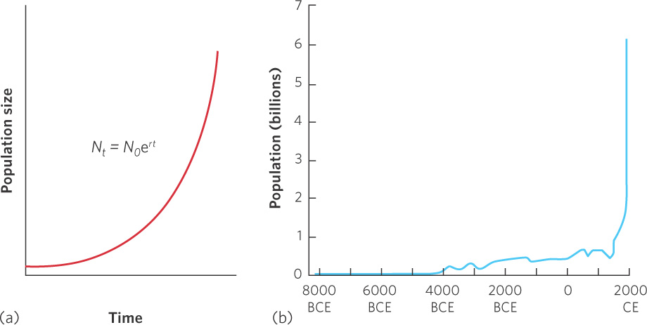
Once we know the intrinsic growth rate for a population, we can estimate how a population will grow over time under ideal conditions. To do this, we can use the exponential growth model, so named because it uses a formula that has an exponent:

where e is the base of the natural log (e = 2.72). This equation tells us that when conditions are ideal the size of the population in the future (N_t) depends on the current size of the population (N₀), the population’s intrinsic growth rate (r), and the amount of time over which the population grows (t).

The exponential growth model demonstrates that populations living under ideal conditions can experience rapid growth that, when graphed, produces a J-shaped curve as shown in Figure 12.1a. Figure 12.1b illustrates that the human population has been growing exponentially during the past 300 years.

Figure 12.1 The exponential growth model. (a) Over time, a population living under ideal conditions can experience a rapid increase in population size. This produces a J-shaped curve. (b) Human population growth is an excellent example of a J-shaped curve.

Data from http://www2.uvawise.edu/pww8y/Supplement/ConceptsSup/PopulationSup/ChartWldPopGro.html.

Using the exponential model, we can also determine the rate of growth at any point in time. To do this, we can take the derivative of the exponential growth equation and obtain the following equation:

where represents the change in population size per unit of time. In words, this equation tells us that the rate of change in population size at any particular point in time depends on the population’s intrinsic growth rate and the population’s size at that point in time. Populations with higher intrinsic growth rates or a larger number of reproductive individuals will experience a greater rate of increase in population size. Another way to think about this equation is that it tells us the slope of the line relating population size to time at any given point. Looking at the graphs in Figure 12.1, for example, the slope of the line is very shallow early in time and becomes very steep later in time. This confirms that the population initially grows more slowly because there is a small number of reproductive individuals, but then grows much faster as the number of reproductive individuals increases.

The exponential growth model for a population resembles the way money grows when it is earning interest in a bank account. The number of individuals in the population is analogous to the number of dollars in your bank account, and the intrinsic rate of growth is analogous to the annual rate of interest. Imagine that you had $1,000 in your account, you received 5 percent annual interest, you never added or withdrew money from the account, and any interest earned would be deposited directly into the account at the end of the year. After 1 year the balance would be $1,050, which is an annual growth of $50. The balance after the second year would be $1,102.50—an annual growth of $52.50. In the tenth year, the annual growth would be $77.57, and in the twentieth year the annual growth would be $126.35. As you can see, a constant interest rate results in an ever-increasing balance. Similarly, a constant intrinsic growth rate results in ever-increasing numbers of individuals in a population and the population experiences exponential growth.

The Geometric Growth Model

The exponential growth model can be applied to species that reproduce throughout the year, such as humans. However, most species of plants and animals have discrete breeding seasons. For example, most birds and mammals reproduce in the spring and summer when there are abundant resources available for their offspring. As an example, let’s look at the California quail (Callipepla californica), a bird from western North America that lays one or two clutches of eggs in the spring. The quail population experiences a large boost in its population size in the spring but then the population slowly declines over the summer, fall, and winter due to deaths. You can see the changes in population sizes in Figure 12.2, where each color in the graph represents the new generation of young quail that are produced each spring. When we examine the pattern of population abundance over several years, we can see that the exponential growth model, which assumes continuous births and deaths throughout the year, does not describe animals such as quail that have a distinct breeding period. For these species, ecologists use the geometric growth model because it compares population sizes at regular time intervals. In the case of the California quail, for instance, the geometric growth model allows us to compare population sizes at yearly intervals.

Figure 12.2 The discrete breeding events of the California quail. Each generation of new quail produced each spring is represented by a different color. Because births only happen in the spring, the growth of the California quail is better modeled by a geometric growth model than by an exponential growth model.

Data from J. T. Emlen, Jr., Sex and age ratios in survival of California quail, Journal of Wildlife Management 4 (1940): 92–99.

The geometric growth model is expressed as a ratio of a population’s size in 1 year to its size in the preceding year (or some other time interval). This ratio is assigned the symbol λ, which is the lowercase Greek letter lambda. A λ value greater than 1 means the population size has increased from 1 year to the next because there have been more births than deaths. When λ is less than 1, the population size has decreased from 1 year to the next because there have been more deaths than births. Because there cannot be a negative number of individuals, the value of λ is always positive.

If N₀ is the size of a population at time 0, then its size 1 time interval later would be:

Next, we can examine how we predict population size after more than 1 time interval. For example, if we wanted to estimate population size after 2 time intervals:

which can be rearranged to

In more general terms, then, we can express the geometric growth model as

where t equals time. Imagine that we start with a population of 100 quail and we have an annual growth rate of λ = 1.5. After 5 years, the size of the population is

Using the geometric growth model, we can also calculate how much the size of a population changes between time intervals. The change in population size from 1 time interval to the next is referred to as ΔN, where Δ, the capital Greek letter delta, means “a change in.” The change in population size is the number of individuals at the end of the interval minus the number of individuals at the beginning of the interval

which can be rearranged to

If we return to our example in which the initial population size is 100 and the annual rate of growth is 1.5, the change in population size after 5 years will be

Comparing the Exponential and Geometric Growth Models

Notice that the equation for exponential growth is identical to the equation for geometric growth, except that e^r takes the place of λ. Thus, geometric and exponential growth are related by

which can be rearranged to

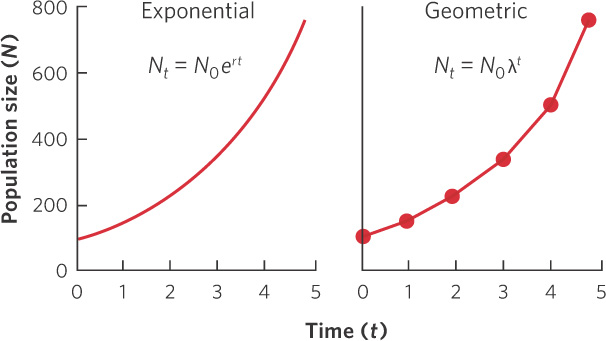
From this relationship, we can see that λ and r are directly related to each other. Indeed, if we were to graph the growth of populations over time using both models and setting λ = e^r, we would find identical growth curves. We see this comparison in Figure 12.3. Although the exponential model has continuous data points whereas the geometric model has discrete data points, the two models show the same pattern in population growth. Figure 12.4 compares the relationships between λ and r by examining the values of λ and r when populations are decreasing, constant, or increasing. When a population is decreasing, λ < 1 and r < 0. When a population is constant, λ = 1 and r = 0. When a population is increasing, λ > 1 and r > 0.

Figure 12.3 Comparing the growth of populations using the exponential and geometric growth models. The exponential model uses continuous data, whereas the geometric model uses discrete data that are calculated at each time point. However, the two models reveal the same increase in population size over time.

Figure 12.4 A comparison of λ and r values when populations are decreasing, constant, or increasing. When the population is decreasing, λ < 1 and r < 0. When the population is constant, λ = 1 and r = 0. When the population is increasing, λ > 1 and r > 0.

Population Doubling Time

We can appreciate the capacity of a population for growth by observing the rapid increase of organisms introduced into a new region with a suitable environment. In 1937, for example, two male and six female ring-necked pheasants were released on Protection Island, Washington. Within 5 years, the population increased to 1,325 adult birds, which means it experienced an annual growth rate of λ = 2.78. In other words, the population almost tripled, on average, each year. Populations maintained under optimal conditions in laboratories can have very high growth rates. Under ideal conditions, the value of λ can be as high as 24 for field voles (Microtus agrestis), a small mouse-like mammal, 10 billion (10¹⁰) for flour beetles, and 10³⁰ for water fleas.

One way of appreciating the potential growth rate of populations is to estimate the time required for a population to double in abundance, known as the doubling time. To understand how we determine doubling time, we can start by rearranging the logistic growth equation:

When a population doubles, its size is twice its original size at time 0. As a result, we can replace (N_t ÷ N₀) with the value 2 and determine the time required (t₂) for a population to double in size:

For the geometric model, the equation is nearly the same, except r is replaced by log_e λ

Given that the value of log_e 2 is 0.69, the doubling time for the ring-necked pheasant, which has an annual growth rate of λ = 2.78, can be calculated as

The same calculation gives doubling times of 79 days for the field vole, 11 days for the flour beetle, and only 3.6 days for the water flea. Using this calculation, demographers have determined that the doubling time for the human population is currently 40 years.

The exponential and geometric growth models are excellent starting points for understanding how populations grow. There also is abundant evidence that real populations do initially grow rapidly, just as these models suggest. As we will see in the next section, however, no population can sustain exponential growth indefinitely. As populations become more abundant, they are limited by other factors such as competition, predation, and pathogens.